Working copy v7 (pre-publish pass done: numbers verified against RESULTS.md M3e–M3g). Math is
$…$/display LaTeX for MDX+KaTeX. The tail notes and this line are stripped by the exporter.
TL;DR. The benchmark-winning way of making an LLM "think harder" (particle filtering on process-reward scores) provably samples the wrong distribution, and in doing so destroys the one signal that tells you when to distrust an answer, irreversibly by the time you can measure it. The mathematics that shows this is seventy years old, and it also supplies the fix: keep 25% of the compute as a never-resampled insurance stratum, which costs no accuracy and restores the signal. Proofs on an enumerable toy model, measurements on real runs, and an interactive replay of the collapse are all below.
I have spent a good part of my PhD being professionally paranoid about samplers. In cosmology, when you infer the composition of the universe from a map of gravitationally lensed galaxies, the answer comes out of a sampler, an algorithm drawing from a posterior nobody can write in closed form. A subtly wrong sampler produces no error message, only a slightly wrong universe with confidently narrow error bars, and you can lose years to a "cosmological tension" that is actually a bug in someone's proposal distribution. So my field grew a culture around one paranoid question: is the sampler actually sampling the distribution it claims to? We have named tests for this (simulation-based calibration, coverage diagnostics), we run them routinely, and a posterior that hasn't passed them is treated as a rumor.
Recently I aimed that paranoia at something far from my field, namely the methods that make a language model "think harder" at inference time. I should be clear about what I am and am not here: I am a cosmologist who knows samplers, physics, and uncertainty quantification, not an LLM researcher, and I walked into the test-time-scaling literature the way a plumber walks into an unfamiliar house, with no opinions about the wallpaper and a professional interest in the pipes. What I found in the pipes is a benchmark-winning method that quietly destroys its own ability to know when it is wrong, in a way the benchmark cannot see, and in a way that turns out to be irreversible by the time anyone looks. None of this has anything to do with language. This post is about that finding, but it is mostly about the dictionary that made the finding cheap: the mathematics on the two sides is the same mathematics, and once you write the mapping down, twenty years of sampler-audit reflexes transfer more or less mechanically.
The dictionary
The LLM setup, which I had to learn from scratch and will compress for anyone else arriving from outside: a generator writes math solutions step by step, a second model (a "process reward model", PRM) scores partial solutions for promise, and search methods use those scores to reallocate compute mid-generation. The benchmark winner, as I write this in mid-2026, is particle filtering (Puri et al. 2025), which runs N attempts in parallel and at every step kills the low-scoring ones and clones the high-scoring ones. Accuracy goes up, and the papers report the accuracy.
Here is what that setup is, translated:
| LLM inference | what it is underneath |
|---|---|
| the base model $p(x_{1:T}) = \prod_t p(x_t\mid x_{<t})$ | an autoregressive reference measure: you can sample it, you cannot renormalize it |
| "generate good solutions" | the tilted measure $\sigma \propto p\,e^{r/\beta}$, i.e. a Gibbs measure, i.e. a Bayesian posterior |
| the process reward model | a learned value function, approximating the optimal "twist" $\psi^\star_t$ |
| particle filtering over steps | Feynman–Kac sequential Monte Carlo |
| best-of-N | the degenerate $T{=}1$ case of the same recursion |
None of these rows is an analogy. The tilted target is a Gibbs measure, the PRM is a value function, the filter is Feynman–Kac, and I have worked with each of these objects under its other name, which is why the audit methodology transfers as machinery rather than as metaphor.
So I did what my field trains you to do and stopped looking at the score, asking instead what distribution the winning method actually samples.
The spine, in five equations
Everything below hangs on what probabilists call Feynman–Kac structure, and the name deserves a short digression, because its origin story is this post's thesis in miniature. Feynman's path-integral picture of quantum mechanics writes an amplitude as a sum over trajectories, each weighted by a factor accumulated along the way. Mark Kac noticed in 1949 that if you run Feynman's clock in imaginary time, the oscillating weights become decaying ones and the construction turns into legitimate probability: an expectation over random walks, with every path multiplicatively reweighted by a potential collected step by step. That pairing of free dynamics with accumulated weights then kept surfacing everywhere. It computes ground states in quantum chemistry as "diffusion Monte Carlo," it models selection acting on lineages in population genetics, and it tracks aircraft as the particle filter, until Del Moral's 2004 book proved these are all one object and gave it the two physicists' names. A language model generating step by step under a reward model's scores is simply the newest instance: the base model supplies the dynamics and the PRM supplies the potential. The mathematics predates the transformer by seventy years and does not care. (For the LLM instantiation see Zhao et al. 2024.)
With the name earned, I will give each piece in its official form and then in words, because the words are where the bug becomes visible.
The target is the reward-tilt of the base model,
$$\sigma(x_{1:T}) \;=\; \frac{1}{Z}\, p(x_{1:T})\, e^{r(x_{1:T})/\beta}, \qquad Z = \mathbb{E}_p\!\left[e^{r/\beta}\right].$$
In words: take every solution the model could conceivably write, and reweight each one by how good its final answer is, with the temperature $\beta$ setting how hard you lean. At large $\beta$ you barely touch the base model, at small $\beta$ you pile everything onto the best answers, and in between you get a distribution that still remembers what a plausible solution looks like while favoring the good ones. The normalizer $Z$ measures how much of the model's probability already sits on high-reward territory, which will matter in a moment. And $\sigma$ is not an arbitrary choice, because it is the unique solution of the KL-regularized control problem
$$\sigma = \arg\max_q \left\{ \mathbb{E}_q[r] - \beta\, D_{\mathrm{KL}}(q\,\|\,p) \right\},$$
that is, the best possible compromise between scoring high and staying plausible. Readers from the alignment world will recognize this as the RLHF objective. Preference training amortizes $\sigma$ into weights while test-time search buys it with compute, so the two are the same target on different payment plans.
There is a structural problem, though: the model writes one token at a time, but the reward only exists at the end. The bridge between them is the optimal twist, the conditional expectation of the terminal potential,
$$\psi^\star_t(x_{1:t}) = \mathbb{E}_{p(x_{t+1:T}\mid x_{1:t})}\!\left[e^{r/\beta}\right], \qquad \psi^\star_t = \mathbb{E}_{p(x_{t+1}\mid x_{1:t})}\!\left[\psi^\star_{t+1}\right].$$
In words, the twist answers the question a chess engine answers about a midgame position: not "was that move good" but "how do games passing through this position tend to end, averaged over the ways the game might continue." It is a value function. The recursion on the right says that today's promise is the average of tomorrow's promise, which is the Bellman equation wearing sampling clothes. And this is the most useful line in the whole dictionary: a PRM is a learned approximation of $\psi^\star_t$. When a reward model scores a half-written solution, it is estimating an average over futures. The entire story turns on that fact.
Given any twist $\psi_t \approx \psi^\star_t$, the proper sequential sampler weights particles by the incremental ratio
$$w_t = \frac{\psi_t(x_{1:t})}{\psi_{t-1}(x_{<t})}.$$
The idea is to charge each step only for the new promise it added. A step that turns a mediocre prefix into a great one pays a large weight, while a step that merely preserves the promise its prefix already had pays nothing, because that promise was priced in at the previous step. Multiply the ratios along a trajectory and everything interior cancels, so by the end each solution has been charged exactly once, for the quality of its final answer. That cancellation is what "targets $\sigma$" means, mechanically. Two classical gifts come free. The normalizer estimate $\hat Z = \prod_t \big(\tfrac1N\sum_i w_t^{(i)}\big)$ is unbiased, and by Jensen the gap $\log Z - \mathbb{E}[\log \hat Z]$ equals the KL divergence from the sampler's law to the target. In words, the sampler carries its own odometer, and the amount by which the odometer under-reads is exactly how far the sampler is from the right distribution. A correctness certificate, built into the algorithm, for anyone who cares to read it.
The benchmark-winning method does something different. It overwrites the weight with the absolute score, $w_t = \psi_t$, and resamples every step, so the product no longer telescopes and the population targets
$$\sigma' \;\propto\; p \prod_{t=1}^{T} \psi_t \;=\; \sigma \cdot \prod_{t=1}^{T-1}\psi_t .$$
Here is the same thing without symbols. The PRM's score of a half-solution already contains the future, since "this looks promising" means "this will probably end well." Resampling on the absolute score at every step therefore charges the population for the same future again and again, the way a billing department might charge you the full annual subscription every month. No single charge looks wrong, nothing crashes, and that is exactly why the bug is invisible from inside. (As a sanity check, at $T=1$ there is only one charge, $\sigma'=\sigma$, and the bias vanishes, which is why best-of-N is innocent. That fact will matter again later.) On a 125-sequence toy model where all of this reduces to finite sums, the overcharge comes out to 0.20 nats with the optimal twist, so the scheme is off target even when the reward model is perfect, which tells you the problem is the scheme.
The sampler runs colder than you asked
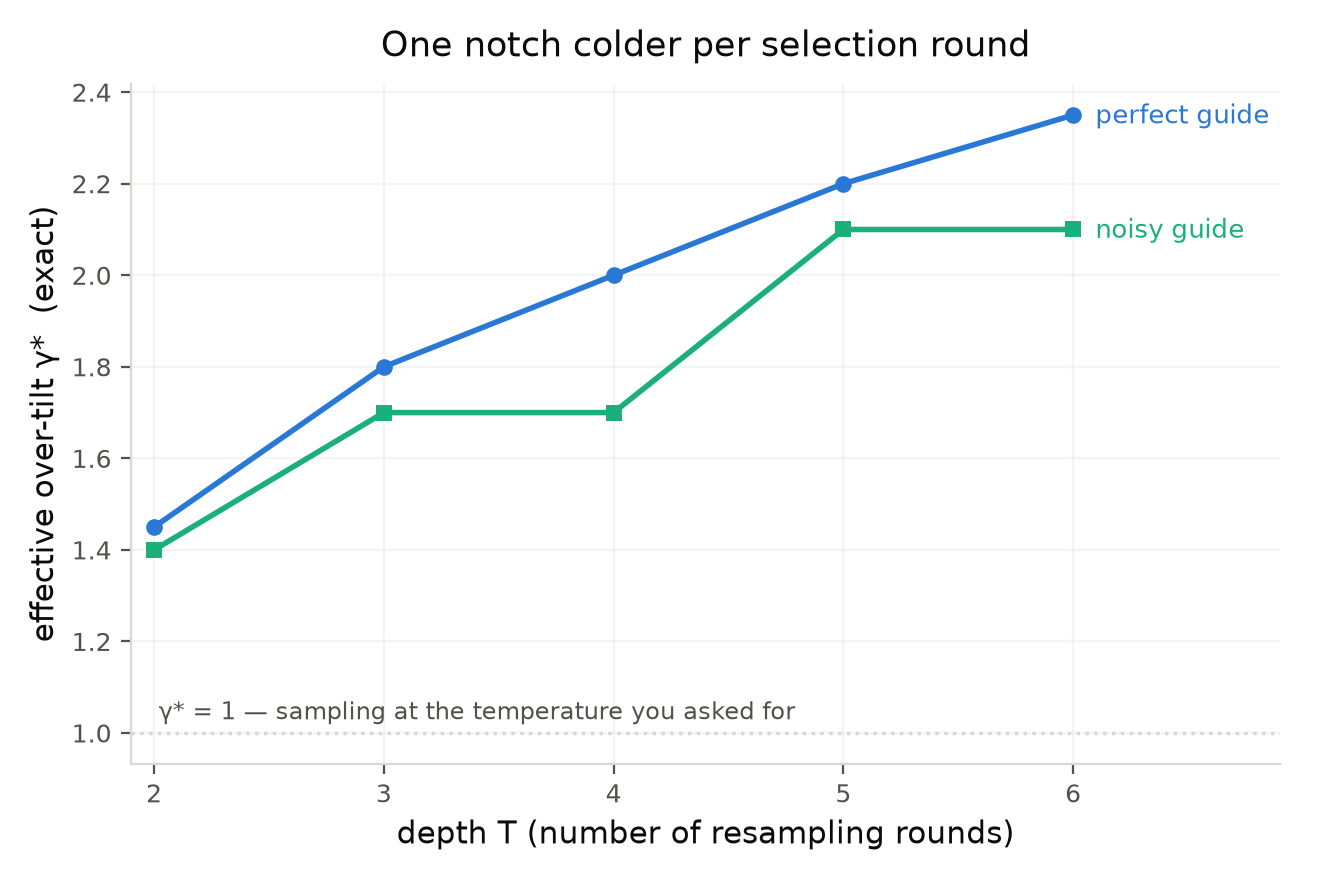
What kind of "off" is $\sigma'$? Fit an effective temperature: find the $\gamma^\star$ minimizing $D_{\mathrm{KL}}\!\big(\sigma' \,\|\, \sigma_\gamma\big)$ over $\sigma_\gamma \propto p\,e^{\gamma r/\beta}$. On the toy model, exactly:
$$\gamma^\star(T) = 1.45,\; 1.80,\; 2.00,\; 2.20,\; 2.35 \quad \text{for } T = 2,\dots,6 .$$
You set the temperature, but the sampler turns the thermostat down another notch with every selection round, and the fit is imperfect in an instructive way, since only about 60% of the divergence is temperature-like and no amount of post-hoc rescaling recovers $\sigma$ either.
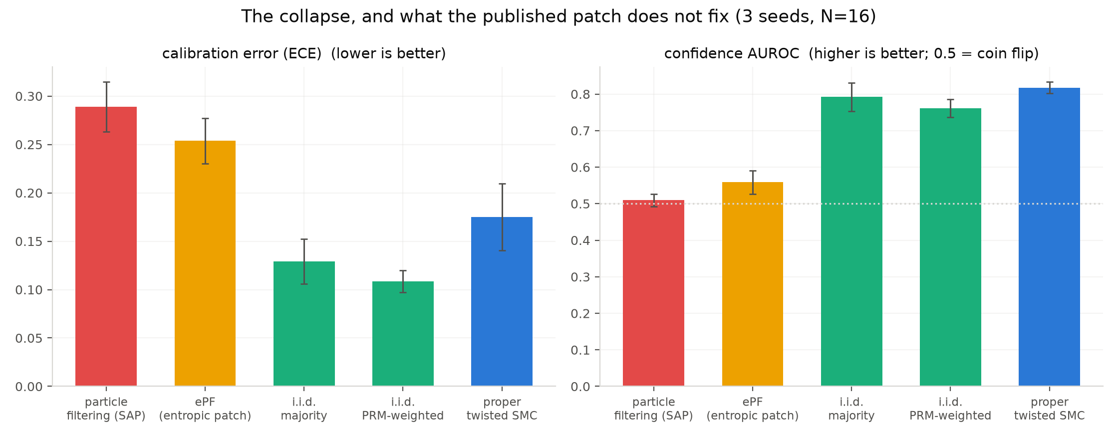
Cold systems concentrate, and the over-cooled sampler collects a little extra reward (mild Goodhart, which the benchmark dutifully rewards) while its answer distribution collapses toward unanimity. That collapse is a calibration catastrophe. Measured on hard MATH problems, across seeds, across budgets $N\in\{8,16,32\}$, and across two models, the winning method reports around 99% population confidence at 65 to 70% accuracy, and its confidence cannot rank its right answers above its wrong ones (AUROC $0.51 \pm 0.02$, which is a coin flip). The identical statistic under plain independent sampling is the standard self-consistency confidence, and it works fine there, with an AUROC around 0.8. The search did not so much miscalibrate the signal as delete it.
Two follow-ups sharpen the point. First, the method's own authors published a diversity-preserving patch (ePF, entropic annealing), built precisely to fight this collapse. We ran it, and it recovers the reward as advertised while restoring none of the signal, with the same collapsed entropy and the same dead AUROC. The patch fixes the symptom its authors were optimizing for, which is fair enough, but as far as I can find, nobody checked the distribution. Second, on a general-purpose model, where the search genuinely buys 13.5 extra points of accuracy over best-of-N, the signal dies exactly the same way. So this is not a no-free-lunch story but a specific bill, itemized to a line of the menu that nobody reads.
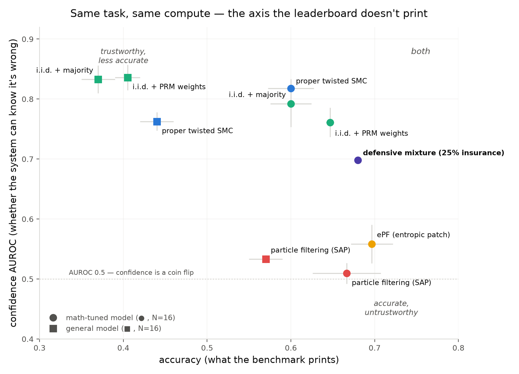
The structural point, stated once: benchmarks are functionals of the argmax while the damage lives in the measure, so an accuracy-shaped scoreboard cannot price the damage, and worse, its gradient points toward the methods that incur it.
Interlude: do we even care about calibration in LLMs?
Fair question, and I want to steelman it before answering, because the answer people usually give ("the literature says calibration matters") convinces nobody. LLMs are mostly used as argmax machines, where the user takes the top answer and applies their own judgment, and nobody inspects a population confidence. On top of that, "calibration" carries a whiff of metric ghetto, a number optimized by people who publish about that number. If your use case is one-shot answers read by a skeptical human, you genuinely don't care, and the over-cooled sampler is even mildly good for you, since its greed buys those few extra points of accuracy.
The real argument has two steps. Step one is a distinction. "Calibration" conflates two properties. One is scale, asking whether the system is right 90% of the time when it says 90%. Scale errors are cheap to fix after the fact (temperature scaling, Platt) because they are a monotone relabeling of an intact signal. The other is rank, asking whether higher confidence actually means more likely right. Rank is measured by AUROC, and rank damage is not fixable afterwards, because no monotone map creates information that isn't there. What the search destroys is rank, so the standard dismissal ("who cares, just recalibrate") fails on the same one-way-door logic as everything else in this post: there is nothing left to recalibrate.
Step two is why rank is where the money is. Any deployment that is not a human reading one answer contains a decision with asymmetric costs, whether that is answering now versus escalating to a bigger model, acting versus verifying first, or auto-accepting versus routing to a person. The optimal policy for every one of these is a threshold on a confidence score, which means the entire value of the system is a function of that score's rank quality. At AUROC 0.5 no useful threshold exists, your options collapse to verifying everything (no automation left) or accepting the full error rate (silent corruption), and the middle ground where deployment actually lives is gone.
Concretely, with our own numbers, on the same 280 problems with the same particle budget and two samplers: play the escalation game, where you may send the fraction $q$ of answers the system is least confident about to an oracle (a stronger model, a human, a verifier) that always gets them right.
| check budget $q$ | search-based winner (acc 67%, AUROC 0.51) | diversity-preserving (acc 61%, AUROC 0.82) |
|---|---|---|
| 0% | 67.1% | 61.1% |
| 10% | 72.9% | 68.9% |
| 20% | 76.0% | 77.1% |
| 30% | 78.9% | 84.6% |
| 50% | 85.0% | 91.1% |
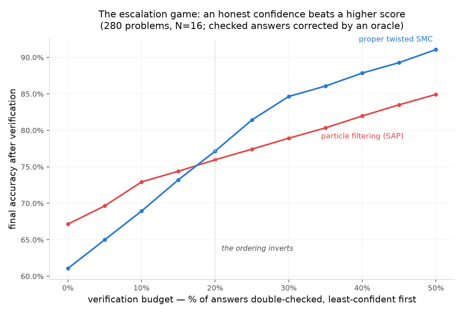
The benchmark winner starts six points ahead, and that opening row is the leaderboard row, the only row a benchmark prints. Give the system any realistic verification budget and the ordering inverts: by $q=20\%$ the "less accurate but honest" sampler has overtaken it, and at 30% it leads by almost six points, because its confidence concentrates twice as many of its errors into the checked pile (41% versus 27% of all errors in the bottom-20% bucket). The two systems solve the same task with the same compute, and their ranking flips the moment they are embedded in any larger process, which in practice means the moment they are deployed.
There is also a version of this that lands close to irony. The premise of the entire test-time scaling field is adaptive compute, the idea that easy problems shouldn't cost what hard problems cost, and so something has to tell you, per problem, whether to stop or spend more. That something is the population's uncertainty, which makes it the fuel gauge of the whole enterprise. With the honest sampler, the dumbest policy I could write (run $N{=}8$, escalate to $N{=}32$ only when confidence is below 0.9) reaches the full flat-$N{=}32$ accuracy at an average of 25 particles instead of 40, so the gauge alone is worth a 37% compute discount. Run the same policy on the benchmark winner and it escalates 4% of problems, because its gauge is pinned at "full" everywhere, and it finishes below its own flat $N{=}8$ accuracy. Aggressive search saws off the branch that adaptive test-time scaling sits on: it always looks done, so it can never tell you where the next particle should go.
The quieter version, for anyone who runs models inside pipelines, is that a component whose outputs carry no trustworthy uncertainty is what an emulator without error bars is in cosmology, unusable at any mean accuracy because you can neither check everything nor check nothing. And notice what the collapsed population physically is: N samples you paid full compute for, reduced to N near-copies of one guess. The uncertainty representation was the thing you were buying with the parallelism, and the search spent it on greed. (The training-time version of the same tilt, RLVR, amortizes that trade into the weights, which is part of why reasoning models volunteer "I'm not sure" about as often as a student volunteers that the exam went badly.)
You can't unburn the toast
My first instinct was the one every importance-sampling person has, which is to reweight, because we are a hammer-rich community. The sampler is off target, fine, but we logged every score it ever used, and the correction is a function of the surviving sequence alone:
$$\frac{d\sigma}{d\sigma'}(x) \;\propto\; \prod_{t=1}^{T-1}\psi_t(x_{1:t})^{-1}.$$
In words, it refunds the double-billed months: divide out every interior charge in one stroke. The correction is computable from the logs with no new generation, and it is algebraically exact, unit-tested by feeding it true samples of $\sigma'$ and watching it recover $\sigma$ on the nose.
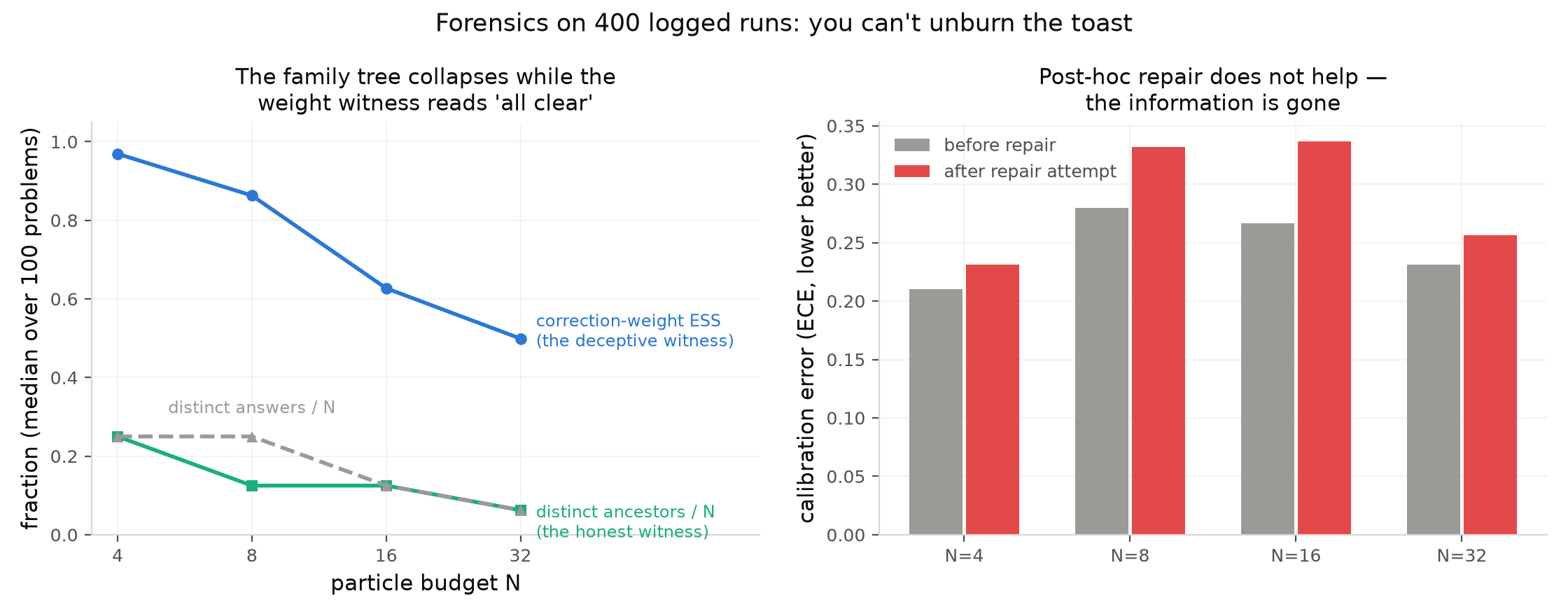
On real logged runs it fails completely, and the reason it fails is the most transferable thing in this project. Any reweighting is bounded by what survived,
$$\mathrm{TV}\big(\text{any reweighting},\, \sigma\big) \;\ge\; 1 - \sigma(\mathrm{supp}),$$
which says nothing more mysterious than that no reweighting can conjure up answers that no surviving particle is holding. And after a dozen winner-take-all rounds the surviving support carries a few percent of $\sigma$'s mass. On the exact toy the corrected estimator lands right on this floor, and on 400 logged production runs the final population typically descends from two or three of the thirty-two starting lineages, which makes it the most confident committee I have ever seen in which everyone is a cousin. Selection does not distort the information, it destroys it. Population genetics has owned this mathematics for a century under the name of genealogical coalescence, and the everyday version is familiar too: no weighting of the people you hired reconstructs the applicant pool.
Two warning lights fall out of the analysis, both computable from logs while the search runs. The ESS of the would-be correction weights catches density distortion, which is the repairable kind, and the count of distinct ancestral lineages catches support destruction, which is not. The subtlety I did not predict, and the detail I would most want an expert to remember, is that on collapsed populations the weight-based light stays green, because the survivors are near-copies whose weights agree, while the family tree underneath is quietly becoming a stump. Watch only the weights and the toast burns with the smoke detector saying "all clear."
The fix is from 1995: buy insurance
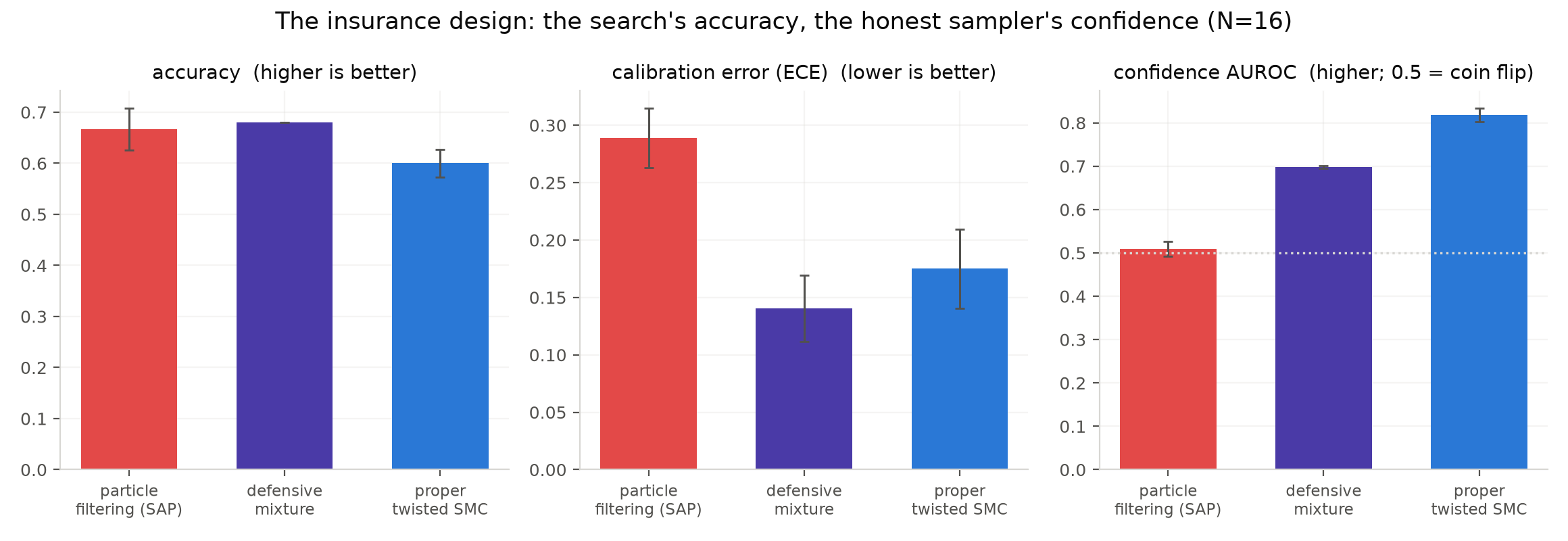
If repair-after is impossible, the protection has to happen during the run. Split the budget so that $(1-\alpha)N$ particles run the aggressive search untouched while $\alpha N$ form an insurance stratum that selection never touches, then take answers from the union, so the search keeps its accuracy, and take confidence from the insurance alone, which the search cannot corrupt. This is defensive importance sampling, old enough to have grandchildren (Hesterberg 1995, Owen and Zhou 2000). With the mixture proposal $q_\alpha = \alpha\, p + (1-\alpha)\, q_{\mathrm{search}}$ the weights are bounded,
$$w(x) = \frac{\tilde\sigma(x)}{q_\alpha(x)} \;\le\; \frac{\tilde\sigma(x)}{\alpha\, p(x)},$$
so the confidence estimator stays consistent with finite variance no matter how pathological the search stratum becomes. In words, because the insurance stratum guarantees every region of answer space a minimum chance of being seen, no single sample can ever matter more than $1/\alpha$ times its fair share, and that bound is what the guarantee is made of. Cosmology runs the same reflex in different clothes, since nobody in my field estimates a correlation function without dragging a catalog of unclustered random points through the identical pipeline. We carry bags of random points around the way other people carry umbrellas, and it looks exactly as silly, right up until it saves you.
Measured at $\alpha = 0.25$ on the real task, the design scores 68.0% against the full-budget search's 68.0%, so the insurance premium costs the selection nothing, to the decimal. Meanwhile the calibration error drops by half (ECE 0.14 versus 0.25 to 0.33) and the AUROC comes back from the dead, from 0.53 to 0.70. The accuracy-or-trustworthiness trade-off the benchmark hides is not a law of nature but a design choice with a known premium, and the premium turns out to be small.
A note for the distribution-free crowd
If your reflex at this point is conformal prediction, meaning wrap the confidence in a distribution-free guarantee and stop worrying about what the sampler did, the finding has an edge for you too. Conformal methods are valid unconditionally, which is their glory, but their efficiency, the set sizes and the selective throughput, is entirely a function of the score's rank quality, and validity without efficiency certifies nothing you can use. On our tables, calibrating a split-conformal selective policy ("answer only above a threshold chosen so selected answers are at least 80% correct") gives the honest sampler a policy that answers 60% of problems at a realized 79%, so the guarantee transfers. On the collapsed sampler the target is unreachable on 92% of calibration splits, because no threshold exists whose bucket clears 80% when the method's most-confident answers are only about 68% correct. The wrapper stays valid, but the policy it certifies is to abstain on essentially everything. Conformal prediction certifies whatever information survives the sampler, and it cannot manufacture information the sampler destroyed, which is this post's only real theme in one more costume. (The natural pairing, for what it's worth, is to conformalize on the insurance stratum, which is exactly the exchangeable, selection-untouched sample a conformal guarantee wants to see. The continuous version of all this, conformalized quantile regression on functionals of steered samplers, belongs to Part 2.)
The principles, without the LLMs
Strip the language models away and the project defends three statements about any system that samples under selection:
- Point-estimate scoreboards select for distributional damage. If the metric is a functional of the argmax and tilting is free, over-tilting is rewarded, and the loss is booked to every downstream consumer of the distribution, on a line the benchmark doesn't print.
- Selection burns evidence at a compounding, quantifiable rate. Each round adds a notch of effective coldness while the genealogy coalesces toward a stump, and past a witness-detectable point no reweighting recovers the target, so the audit has to happen during the run, because afterwards is arithmetic on ashes.
- The untilted control sample is not optional. A small stratum kept outside the selection process is what preserves a system's ability to know when it's wrong, and at least here it came free.
None of this is new mathematics, which is exactly the point. It comes from statistical mechanics, population genetics, and survey methodology, fields that live and die by stochastic simulators and that spent decades building the distributional reliability practice LLM inference is currently rediscovering one silent failure at a time. The translation is not a metaphor but a short table and the will to take it literally.
Honest boundaries
Everything here is one generator family (Qwen2.5, math-tuned and general variants), one PRM, MATH-500 level 4 and 5 (plus AIME at small n), and N up to 32, so it is a worked example rather than a survey. The exact statements (wrong target, depth law, repair floor) live on an enumerable toy, because that is where ground truth exists, and every real-task claim is a label-based measurement chosen to need no ground-truth posterior. The insurance design's AUROC recovers to about 0.70 rather than the 0.75-plus of fully diversity-preserving sampling, since a four-particle stratum quantizes the confidence. And the deepest limitation motivates the sequel: on language tasks there is no exact posterior anywhere, so verification ultimately leans on the toy. The natural home for this style of audit is a substrate where ground truth is computable at scale. I happen to work with such substrates every day. They are called physical simulators, and that is Part 2.
One more boundary concerns the author. I am not an LLM researcher, and it is entirely possible that parts of this post read naively to people who live in that literature, in which case I would genuinely like to hear where. The bet this post makes is narrower than expertise: it is only that the sampler mathematics does not care which field it runs in.
Code, logged runs, the interactive replay, and every number in this post: github.com/AndreasTersenov/particle-reasoners. Machinery: Del Moral (2004), Zhao, Brekelmans, Makhzani and Grosse (2024), Talts et al. (2018), Lemos et al. (2023), Hesterberg (1995), Owen and Zhou (2000), Puri et al. (2025), Giannone et al. (2025, ePF).