Do Baryons Break Higher-Order Statistics? · The Non-Gaussian Universe 2026

Jun 16 2026 · The Non-Gaussian Universe · FORTH, Heraklion

Can we trust higher-order weak lensing?

Baryonic robustness, and learned vs analytical summaries

Andreas Tersenov · FORTH · U. Crete · CEA Paris-Saclay · slides: andreastersenov.github.io/talks/

§0 We are all optimizing statistics; the two-point camp still does not trust the contours

🧐

the 2-point camp

"I don't believe any of your contours."

what would make HOS flagship-grade?

blinding
robust covariance
emulators
systematics
analytical cross-checks
non-Gaussian likelihood
method limits
null / validation tests
simplicity

Part 1 of 2

Do baryons break HOS?

Baryonic feedback, the wavelet ℓ1-norm, and the BNT transform.

§1 Stage IV is no longer statistics-limited, it is systematics-limited

to trust a statistic

Before we trust any summary statistic, we have to quantify how each systematic affects it, and at the contour level (the inferred parameters).

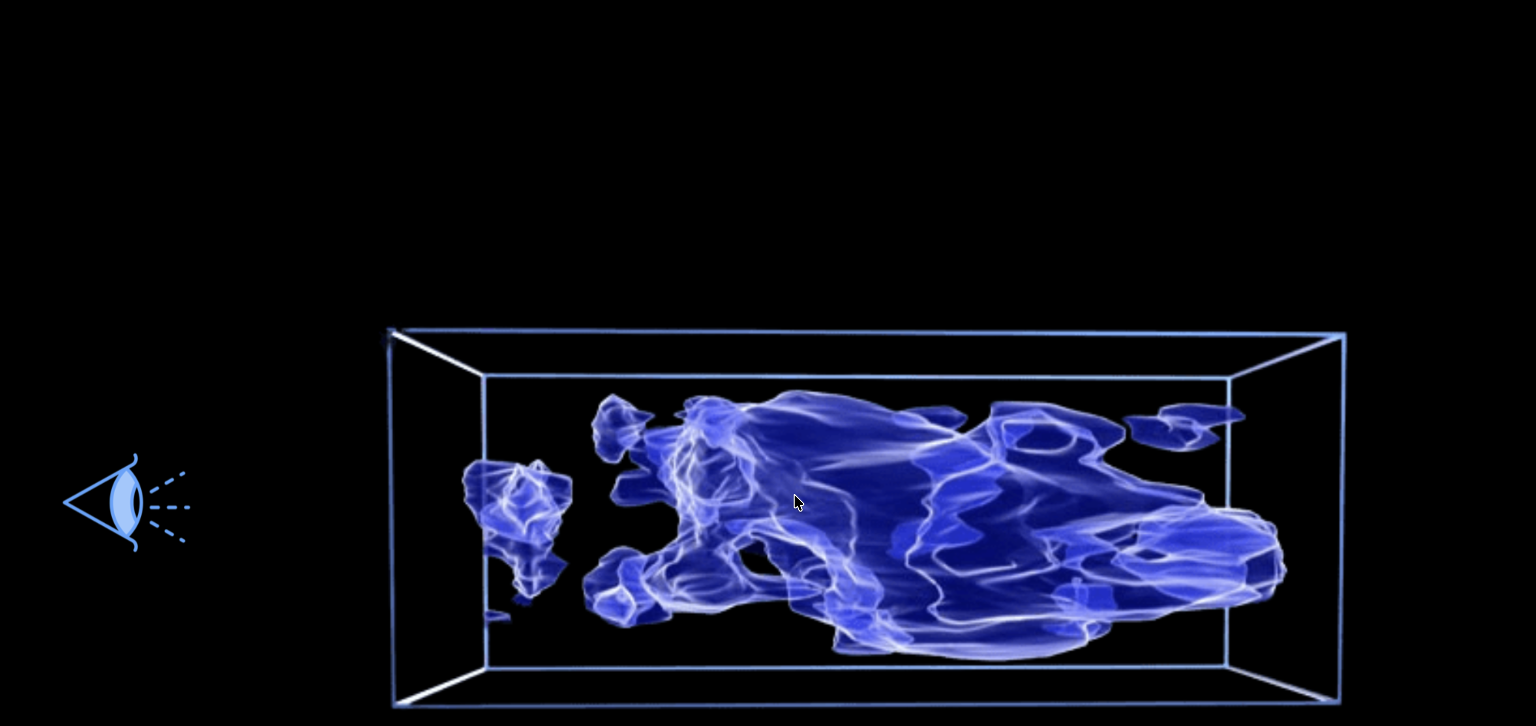
Illustris: baryonic feedback reshaping the cosmic web

the systematic at hand

Baryonic feedback (AGN, supernovae) suppresses matter on small scales, mimicking cosmological signal and biasing inference, exactly where the constraining power lives and where the feedback models disagree most.

core questions

How does unmodeled baryonic feedback bias our non-Gaussian statistics?
After safe scale cuts, do HOS still outperform the power spectrum?

§1 Higher-order statistic I: peak counts

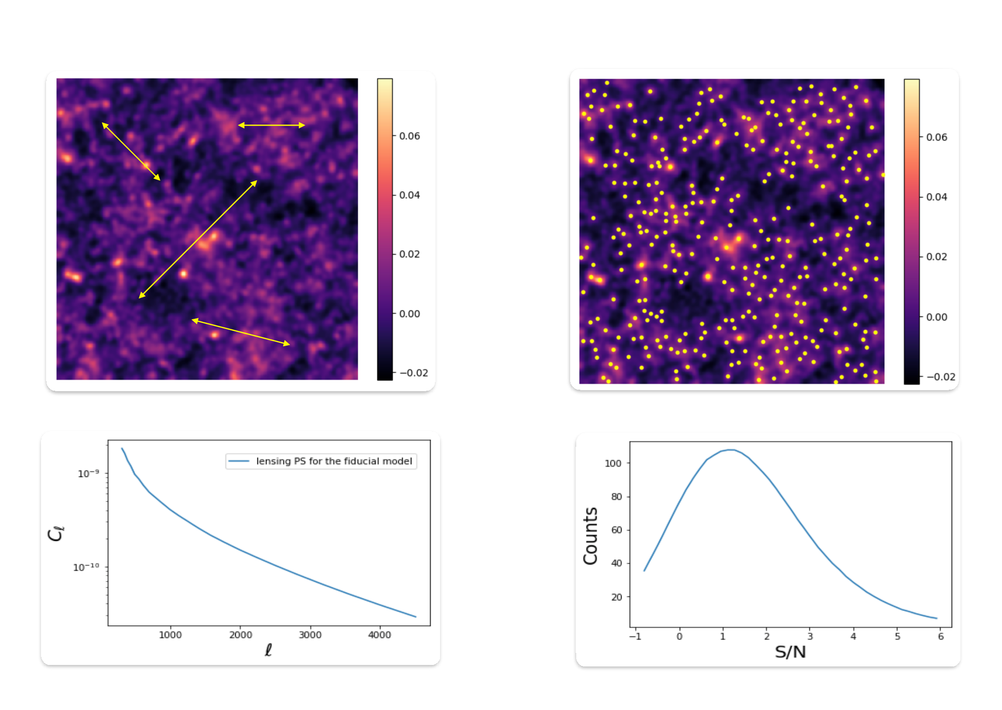
convergence maps with peaks marked, the lensing power spectrum, and the peak-count curve

Peaks: local maxima of the SNR field $\nu = (\mathcal{W} \ast \kappa)(\theta_{\rm ker})\,/\,\sigma_n^{\rm filt}$
Counted per SNR bin; they trace massive structures
Simple and well-established, but uses only the high-SNR peaks

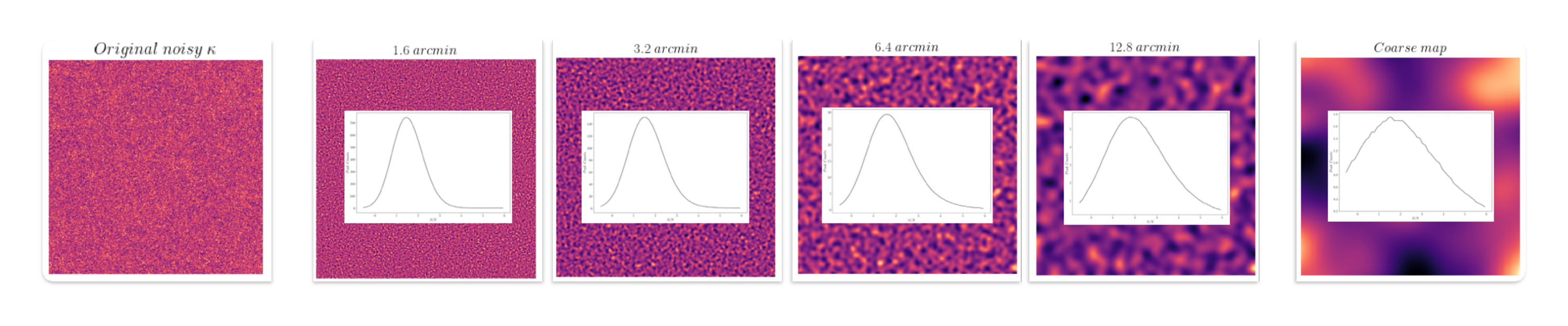
§1 Wavelet peaks: a multi-scale peak count via the starlet transform

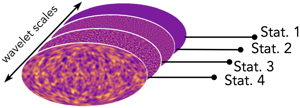
starlet decomposition: a map as a sum of wavelet bands plus a coarse map

Multi-scale, not single-scale
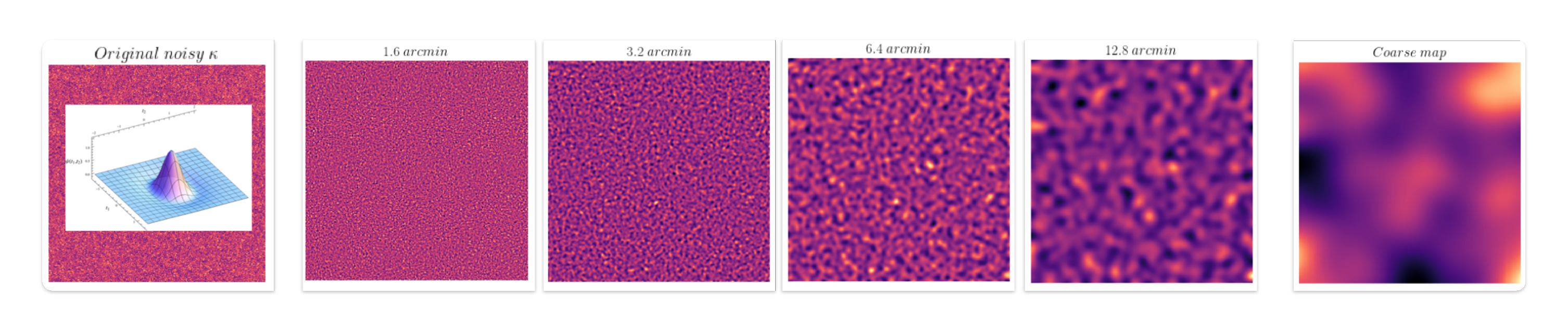
Starlet transform: a map as a sum of wavelet-coefficient images plus a coarse map
Processes all scales simultaneously, for efficiency
Each band is a different frequency range, so the peak-count covariance is nearly diagonal

§1 Higher-order statistic II: the starlet ℓ1-norm

starlet decomposition of a convergence map across scales

$$ \ell_1^{\,j,i} \;=\; \sum_{u} \left| \mathcal{S}_{j,i}[u] \right| \;=\; \lVert \mathcal{S}_{j,i} \rVert_1 $$

Sum of absolute starlet coefficients, per scale and SNR bin
A fast, multi-scale measure of the full void and peak distribution
Information in all pixels: peaks and voids, the full convergence PDF
No discrete-feature definition

The inference pipeline: neural posterior estimation

wavelet-scale maps and summary statistics

+ noise
wavelet transform

condition

Gaussian$\mathcal{N}(0,\mathbf{1})$

Density estimatorconditional MAF

Posterior$p(\theta\mid x)$

training objective

$\mathcal{L}=-\log p_\phi(\theta\mid x)$

§1 Mitigation: Scale Cuts

Goal: bring tension below 0.3$\sigma$
$C_\ell$: requires an aggressive cut at $\ell \lesssim 400$ → discards most signal
Starlet: contamination isolated in one scale → removing just the finest wavelet band is sufficient across all survey areas

parameter tension versus upper scale cut, for different survey masks

We run this analysis as a function of survey area: more area means smaller statistical errors, and thus higher sensitivity to bias.

§1 Baryonic Bias Scales with Survey Area

parameter tension in sigma versus survey area for all statistics

At 14,000 deg² (Stage IV): $C_\ell$ already shows $\sim 2\sigma$ tension
At full sky: tension exceeds $3\sigma$ for all statistics
HOS show higher bias than $C_\ell$: more sensitive to the baryonically-contaminated small scales

power spectrum posterior contours, biased by baryons, for different survey areas

§1 Are HOS still useful?

On baryon-safe scales

Starlet $\ell_1$-norm yields constraints $3\times$ tighter than $C_\ell$ in the full-sky limit
HOS still useful: non-Gaussian signal persists even after the fine-scale cut

Takeaway

Baryonic effects are a dominant systematic, biasing parameter estimation
HOS are not merely deep-non-linear probes: they robustly recover information on quasi-linear scales

§1 But could we do better than that? Weak lensing tomography

the source galaxies as tomographic convergence maps, one per redshift bin

Credit: Justine Zeghal

§1 The BNT transform localizes each tomographic bin in redshift (a linear nulling)

standard lensing efficiency kernels: broad and overlapping across redshift — standard: broad, overlapping

→

BNT lensing efficiency kernels: nulled and localized per bin — BNT: nulled, localized

what BNT does · Bernardeau, Nishimichi & Taruya 2014

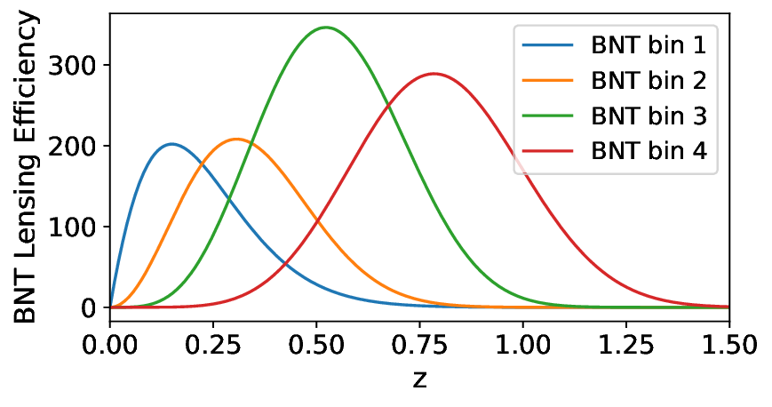
A linear, invertible nulling of the tomographic bins
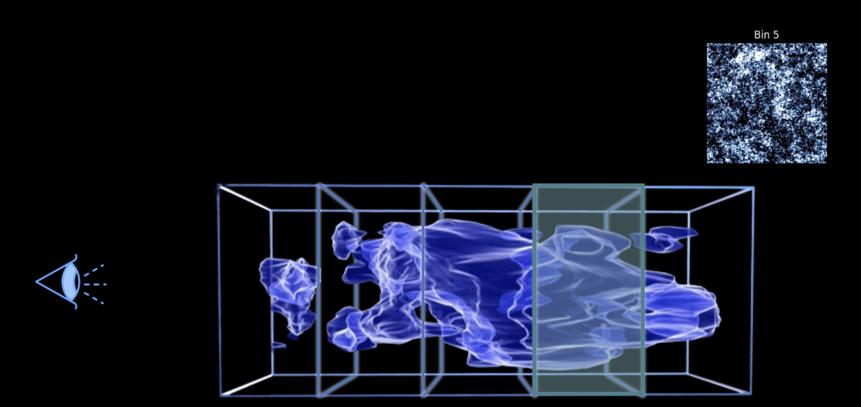
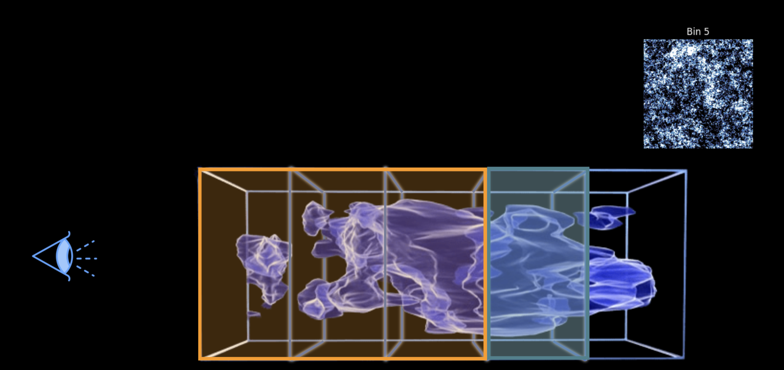
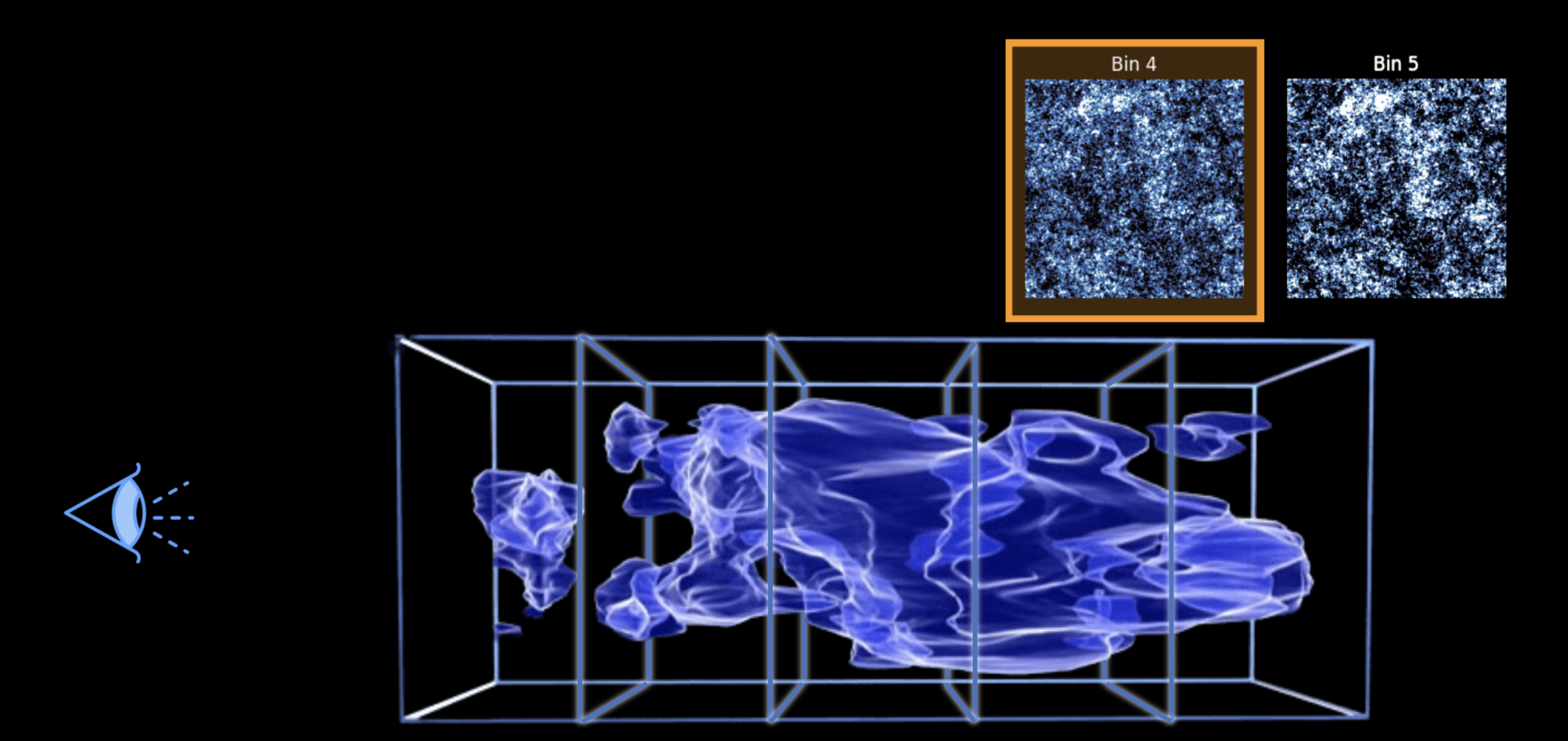
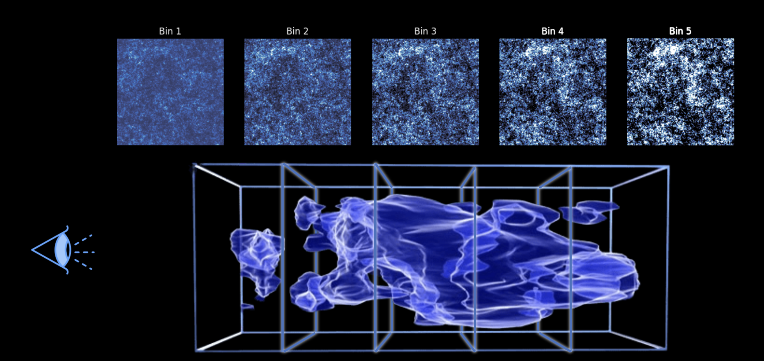
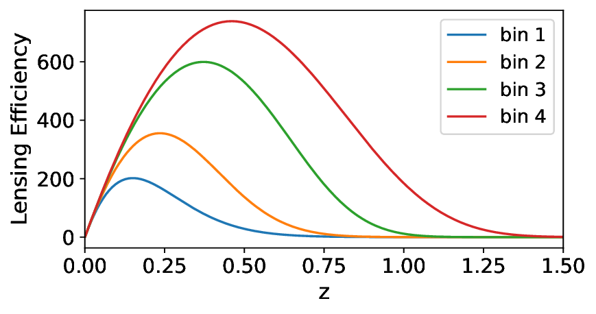
Standard kernels are broad and overlapping, so a fixed angular scale ℓ mixes many physical scales and redshifts
BNT nulls the low-z lensing efficiency, localizing each field in redshift (thin lens-z slices), which sharpens the angular-scale ↔ physical-scale mapping for clean scale cuts

Our use here: isolate the low-z, small-scale systematics (baryonic feedback) to specific bins, and cut scales only where needed, instead of discarding data everywhere.

The BNT transform (Bernardeau, Nishimichi and Taruya 2014) is a linear, invertible nulling scheme that reorganizes the tomographic data into redshift-localized fields. Standard lensing kernels are broad and overlapping, so a fixed angular multipole mixes physical scales and redshifts (low-z non-linear with high-z linear). BNT subtracts weighted lower-redshift bins to null the low-z lensing efficiency, de-projecting the signal so each transformed field probes a narrow lens-redshift range; this sharpens the angular-scale to physical-scale mapping and enables targeted scale cuts. It is a general technique (dynamics, geometry, systematics, nonlinear-scale control); we use it here to isolate low-z baryonic feedback. For the power spectrum it is effectively lossless with the full cross-covariance; for map-based HOS it backfires (next slide).

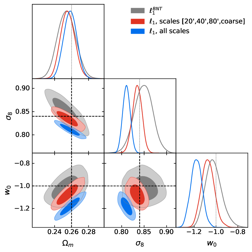
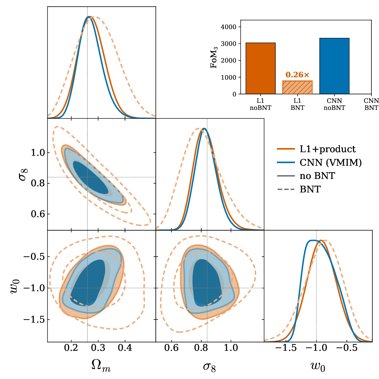
§1 But applied to map-based HOS, BNT inflates the per-bin contours

l1-norm contours: BNT inflated versus safe-scale and all-scale — The per-bin HOS contours **inflate dramatically** (gray = BNT; the noise mixing raises the floor).

the hinge

BNT is invertible: no information can truly be lost
Yet a Euclid forecast (Vinciguerra et al. 2026) still saw inflated BNT contours, even with explicit cross-bin HOS; recovering the SNR is "highly non-trivial"
Is the information really lost, or are we just analyzing it wrong?

Part 2 of 2

Learned vs analytical,
and can we trust it?

The analytical ℓ1-norm vs a learned CNN, calibration, and the answer to the BNT puzzle.

§2 Part 2: learned summaries, and the BNT cliffhanger

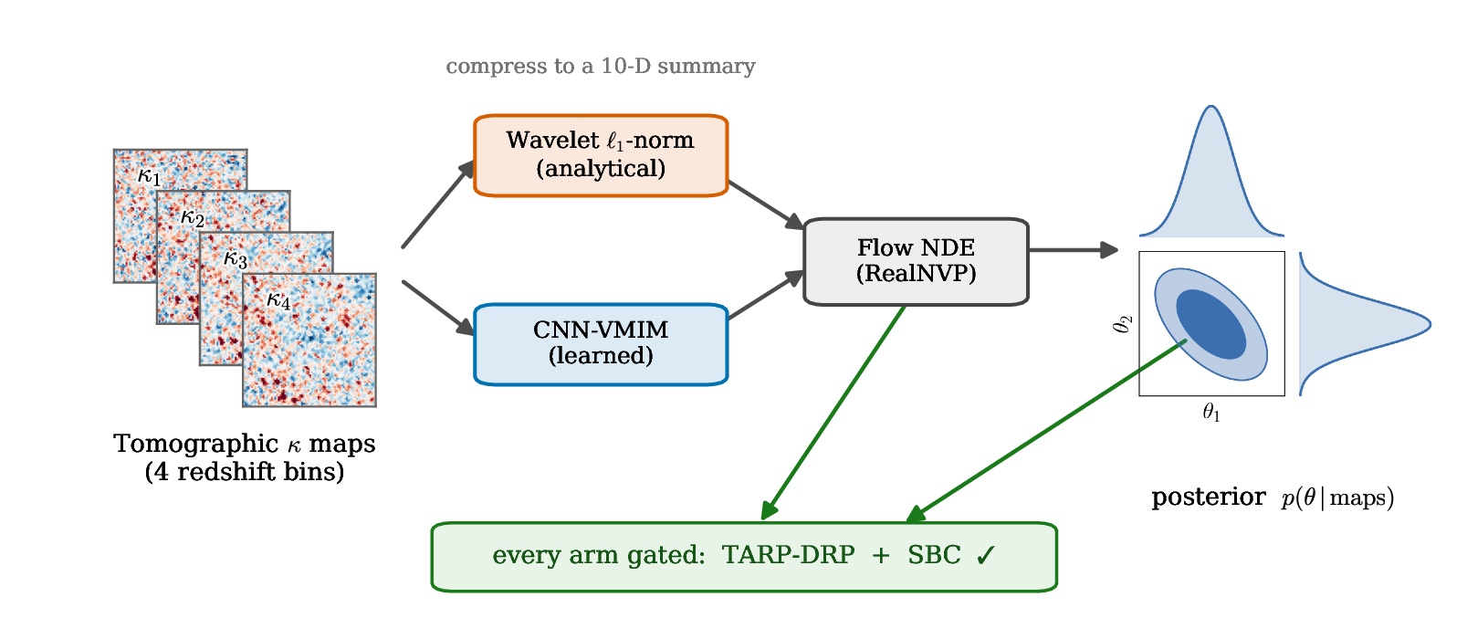
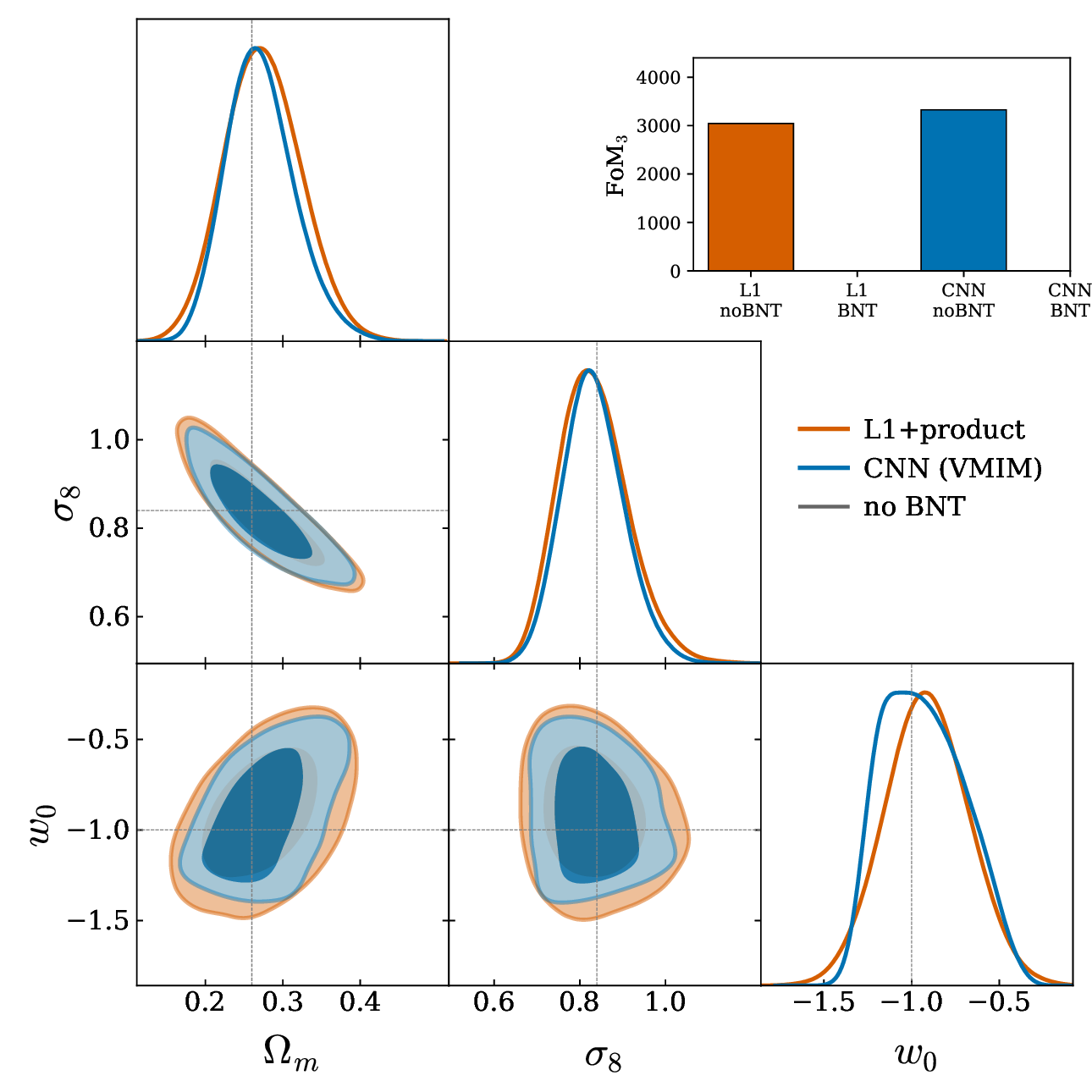
the question How much better are "optimal", learned summaries than our hand-built summary statistics?

what is a learned summary?

A neural network that compresses the κ map directly into a few numbers, instead of a hand-designed statistic
Trained with VMIM to keep the cosmological information: the "optimal learned compressor"

and, left over from Part 1 ...and what the hell is going on with BNT?

Training a neural summary I: regression (MSE)

simulator

$\theta\sim$ prior

→

map $x$

→

network

$f_\phi$

→

estimate

$\hat\theta$

\[\mathcal{L}=\mathbb{E}\,\big\lVert\,\theta-f_\phi(x)\,\big\rVert^{2}\]

parameter space $\theta$

Training a neural summary II: VMIM

simulator

$\theta\sim$ prior

→

map $x$

→

network

$f_\phi$

→

summary

$t$

→

flow

$q_\psi(\theta\mid t)$

→

posterior

$p(\theta\mid t)$

\[\max_{\phi,\psi}\; I(t;\theta)\;=\;\max_{\phi,\psi}\;\mathbb{E}\,\log q_\psi\!\big(\theta\mid f_\phi(x)\big)\]

parameter space $\theta$

§2 The comparison, done fairly: same maps, same flow, both calibrated

kappa maps to either l1-norm or CNN-VMIM, into the same flow density estimator, to a calibration-gated posterior

apples to apples

Same κ maps → ℓ1-norm or CNN-VMIM → the same flow NDE → posterior
Flat-sky 10° patches (cross-maps physically buildable), both arms calibrated
324k patches, 899 cosmologies

§2 The analytical ℓ1-norm almost reaches the optimal CNN (~7%): The hand-built ℓ1+product is near-sufficient

matched-NDE L1+product posterior, with the FoM3 inset

L1 and CNN matched-NDE posteriors nearly coincide (~7%)

ℓ1 and CNN posteriors nearly coincide

per-patch FoM3 distribution for L1+product versus CNN: medians 3045 and 3326, near-identical spread

near-identical FoM3 across patches (3045 vs 3326)

§2 Can we trust it? Every arm passes the same TARP + SBC tests reasonably

TARP-DRP coverage on the diagonal for both arms — TARP-DRP coverage: on the diagonal

SBC rank uniformity within the band for both arms — SBC ranks: flat within the 99.5% band

tight is not the same as correct

Both arms pass the same battery: varied-θ TARP-DRP coverage + SBC rank uniformity
The constraining power is real

§2 BNT revisited: the per-bin ℓ1 collapses (0.26×), the channel-mixing CNN is lossless (0.96×)

the per-bin L1 balloons under BNT (0.26x)

the channel-mixing CNN stays tight under BNT (0.96x)

Same transform, opposite fates

Per-channel ℓ1+product collapses: 3045 → 779 (0.26×; σ₈ +65%)
Channel-mixing CNN is lossless: 3326 → 3186 (0.96×)
The collapse is itself calibrated: a real loss

Same information, a different frame: why BNT collapses the ℓ1-norm but not the CNN

the point cloud (all the information) never moves

lensing kernels q(z)

Signal & noise under BNT: who can read it

noise covariance

What survives BNT: the 2-point rule

§2 Is the +7% worth it? The honest cost of going neural (an open question for the round table)

the benefit

~7%

FoM3 gain of the optimized CNN over the analytical ℓ1, both calibrated.

the cost

extensive architecture and hyperparameter search
a very large dataset (899 cosmologies, ~324k maps); VMIM needs the scale or it biases
unphysical-information traps (patch geometry, map-mean / mass-sheet mode, 20° projection features) that tighten contours dishonestly
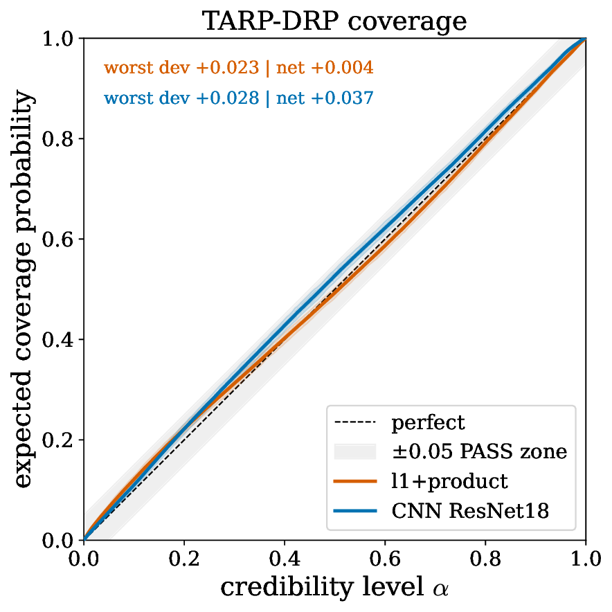
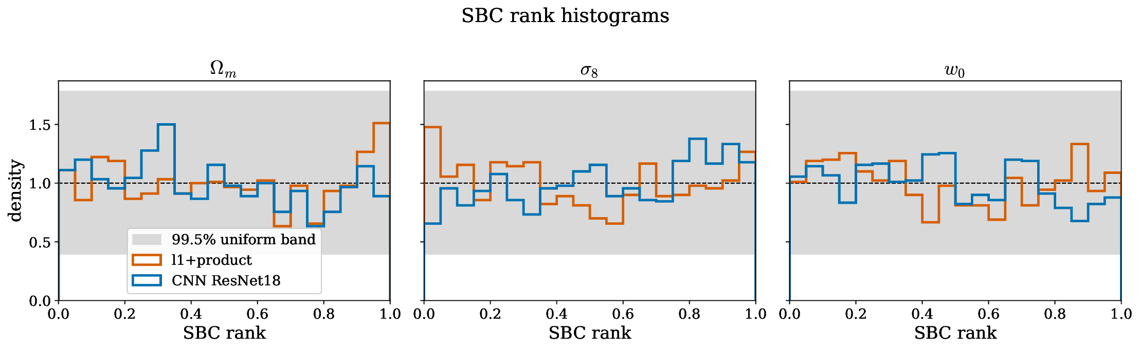
and these largely escape TARP and SBC: the contours look calibrated and are still wrong

the thumb on the scale

ℓ1 is simple, interpretable, inspectable; CNNs are powerful but treacherous
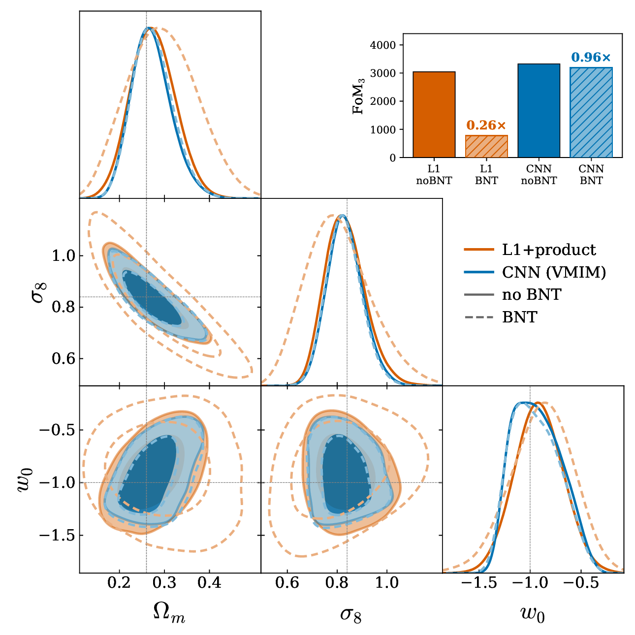
Where the CNN earns its keep: BNT, the channel-mixing win
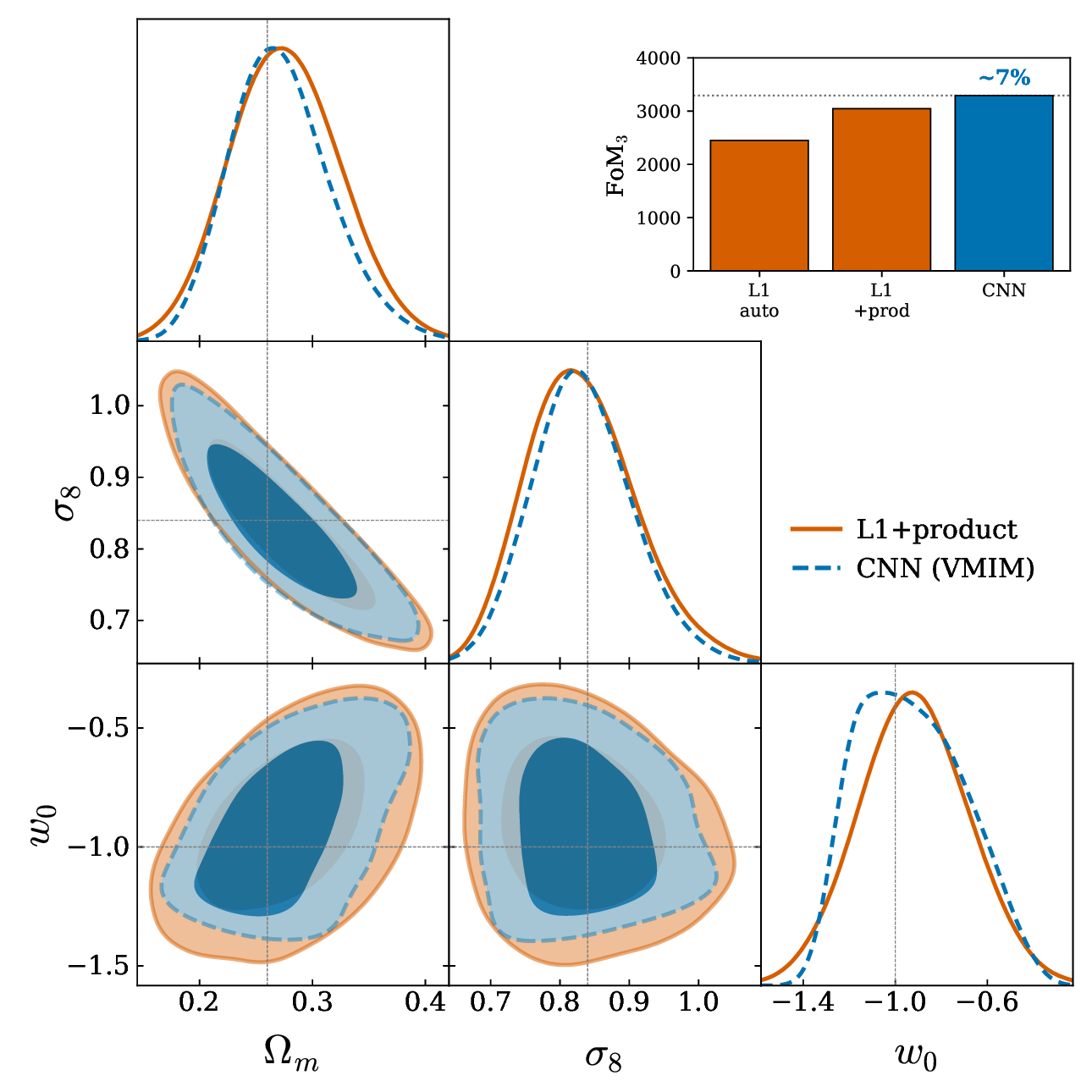
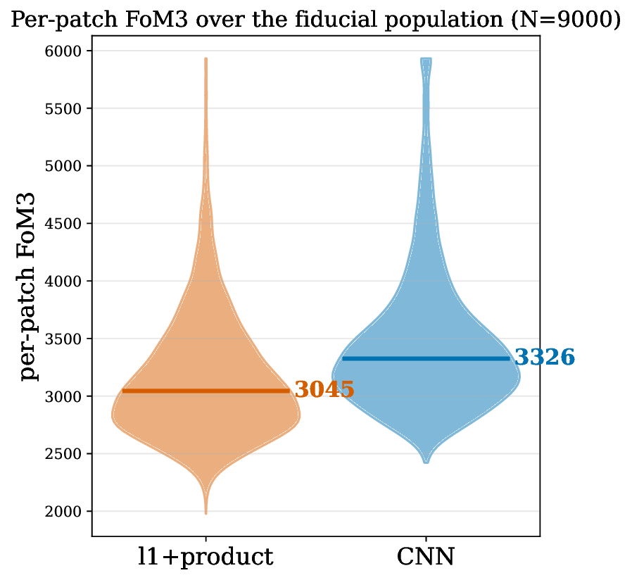
For the panel: is a ~7% gain worth that cost and that risk?

§3 Do baryons break HOS? No.

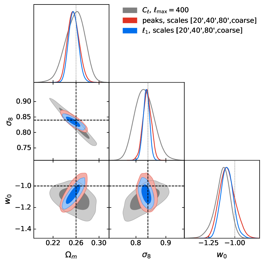
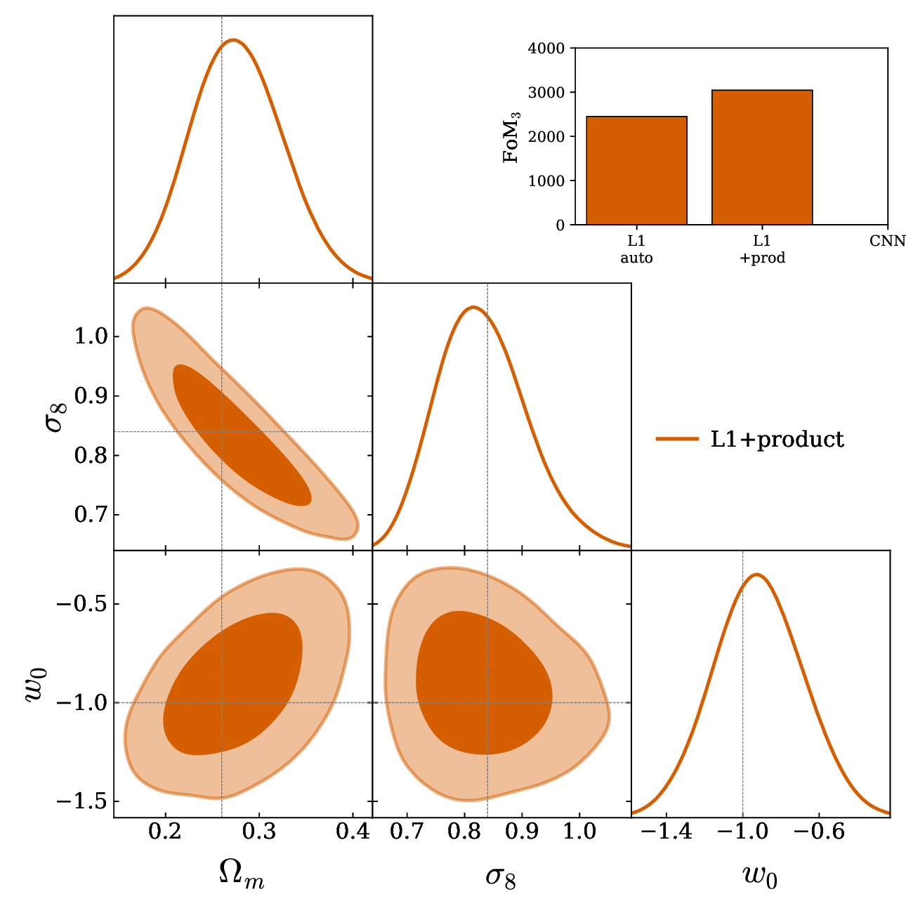
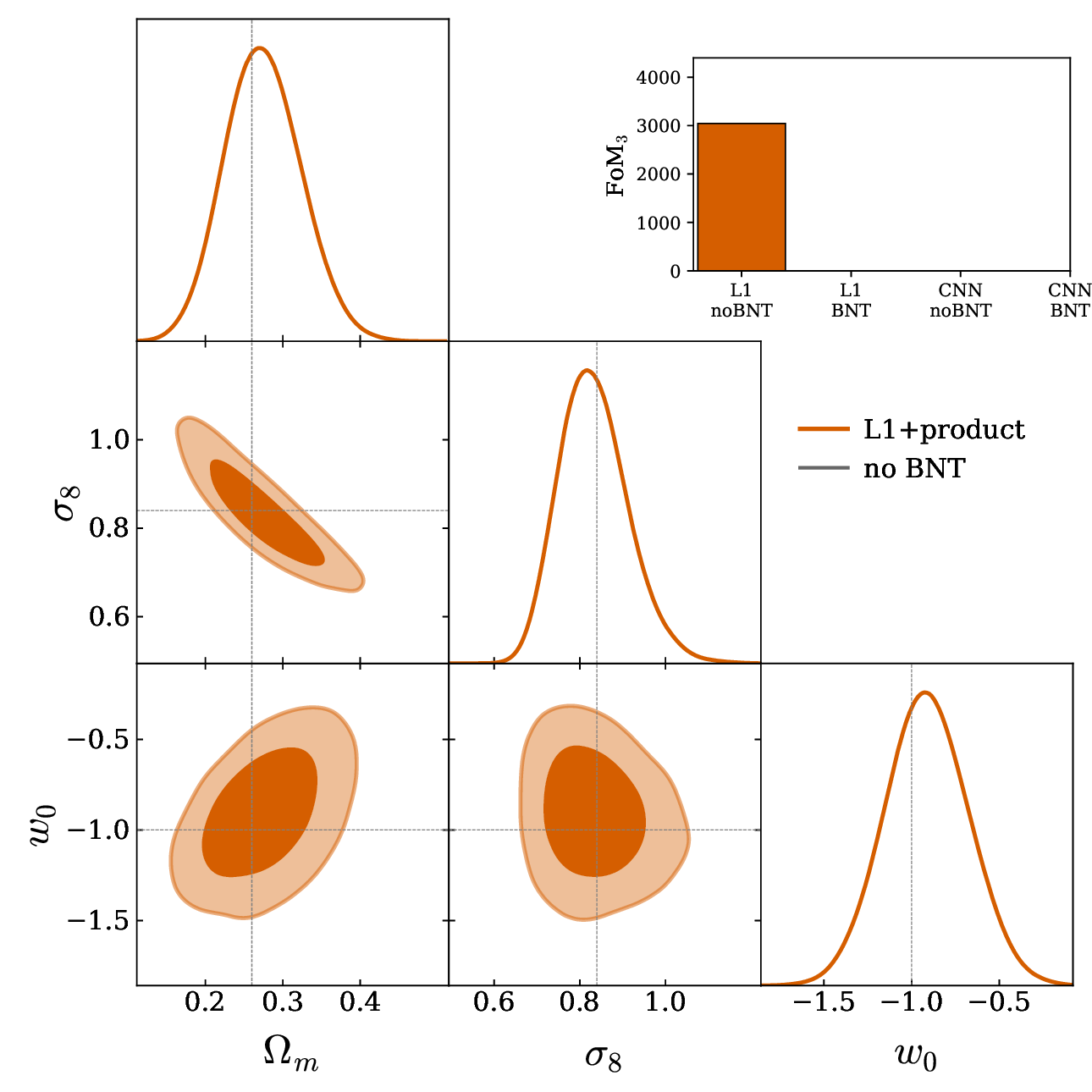
Part 1 · baryons Usable non-Gaussian information persists on baryon-safe scales (the ℓ1-norm beats P(k) ~3×), cleaned by a single scale cut.

Part 2 · learned vs analytical The hand-built ℓ1-norm nearly matches the optimal learned summary (~7%), and both are calibrated.

BNT The apparent BNT break is a frame artifact: a channel-mixing compressor, or one fixed rotation, recovers it.

the bigger question And can we trust higher-order weak lensing? Getting there...

Appendix

Backup

Supporting slides, for questions.

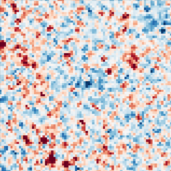
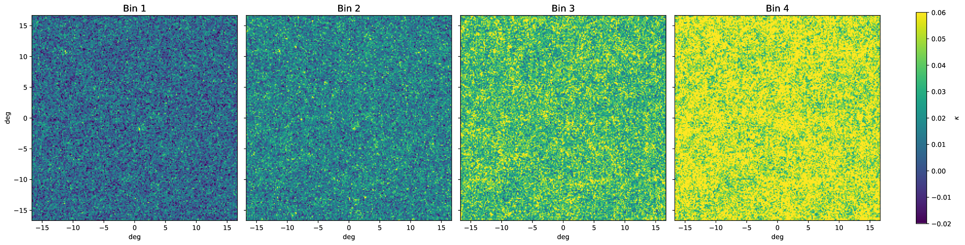
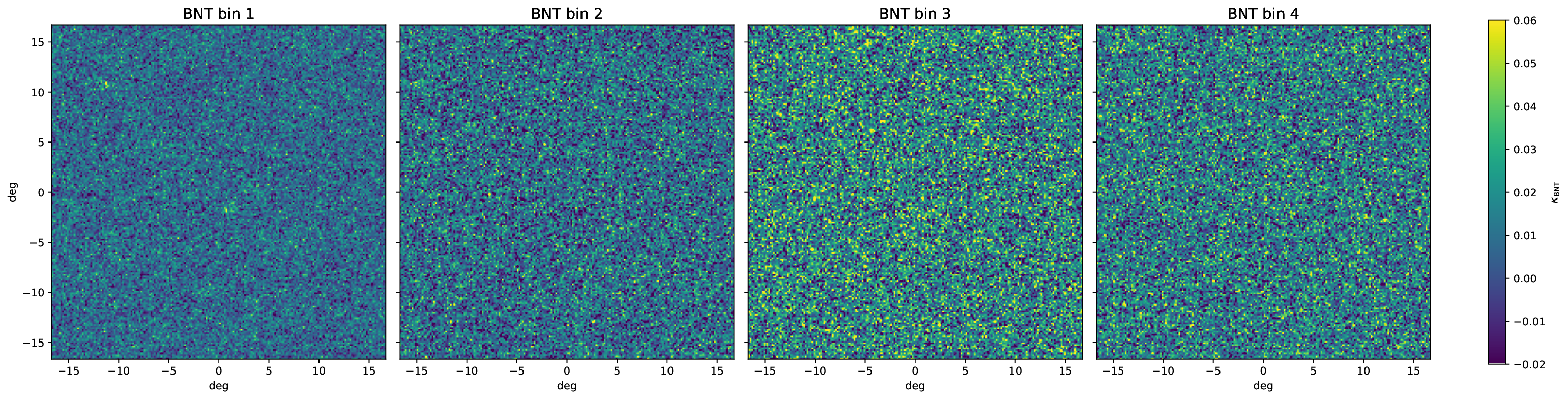
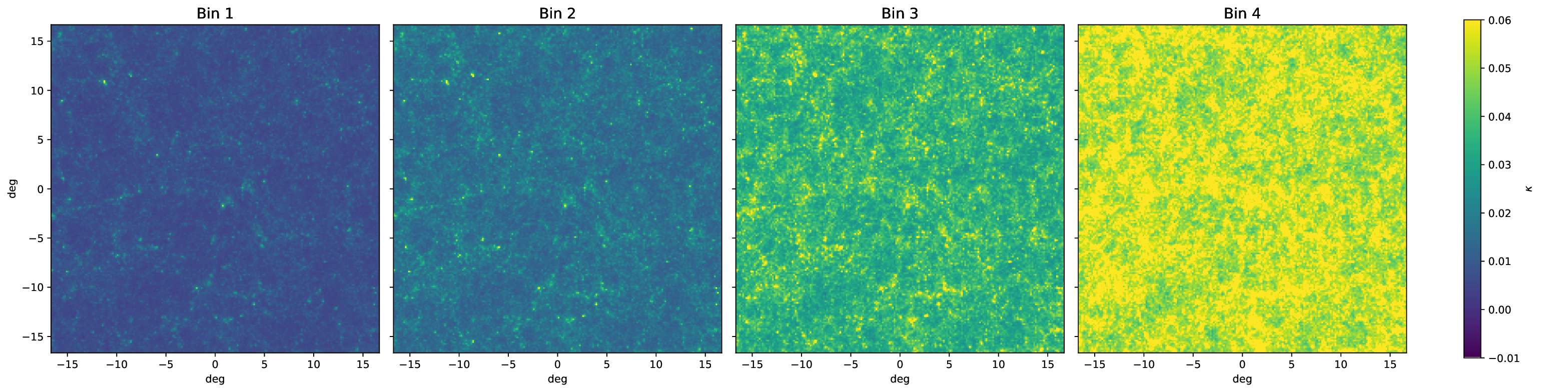
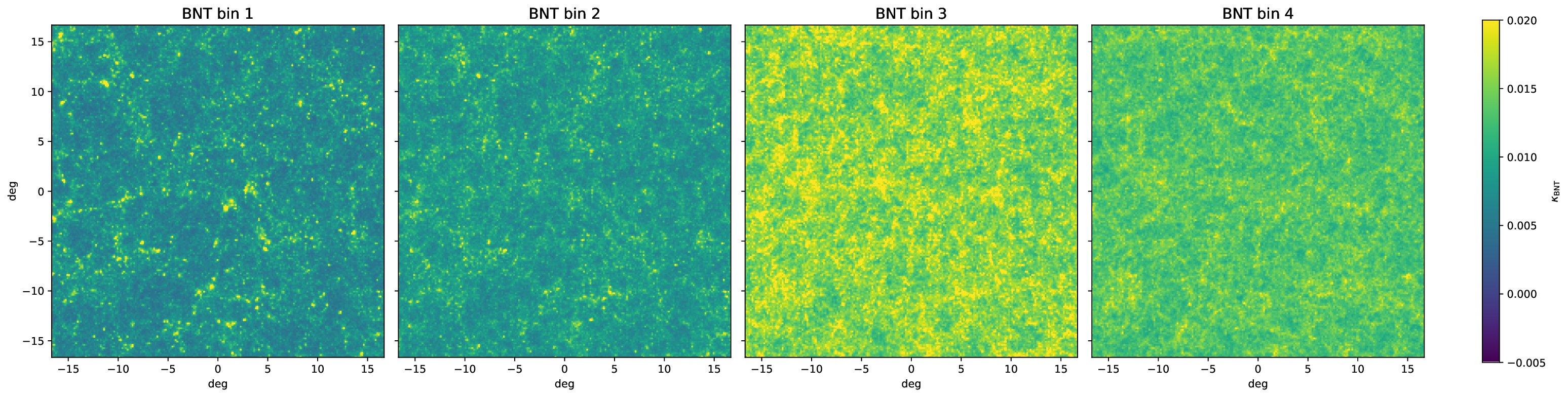
§1 You can see it in the maps: BNT trades deep signal for amplified, correlated noise

noisy tomographic maps before BNT — before BNT

noisy maps after BNT, visibly degraded SNR — after BNT: the SNR collapses

§1 The same maps, noiseless: BNT cleanly redistributes the signal

noiseless tomographic maps before BNT — before BNT (noiseless)

noiseless maps after BNT — after BNT (noiseless)

Without shape noise, BNT is a clean, invertible redistribution of the signal (the deep common mode becomes one shallow map plus thin slices). The contour inflation comes from the correlated noise it introduces, not from any lost signal.

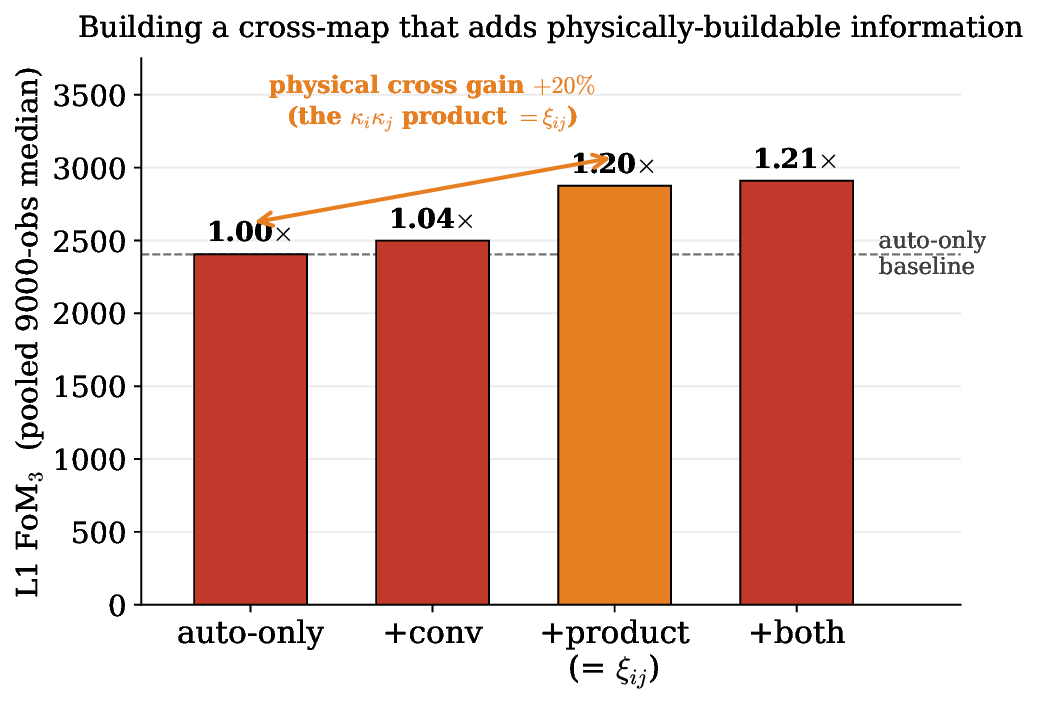
§2 Where the cross-bin information lives: the κ_iκ_j product buys ~20% (and the full-sphere 4× was leakage)

L1 cross-map arms: auto, plus conv, plus product, plus both (no full-sphere bar)

add the cross-bin physics carefully

Product κ_iκ_j (= ξ_ij): +20%
A convolution buys ~0; both together, +21%
The robust, physical cross-bin gain is ~+20%

Community caution: a full-sphere cross construction would inflate this to ~4×, but ~92% of that is leakage (each cross-patch pixel is a global functional of the whole sky). We use only the physically buildable flat-sky arms.

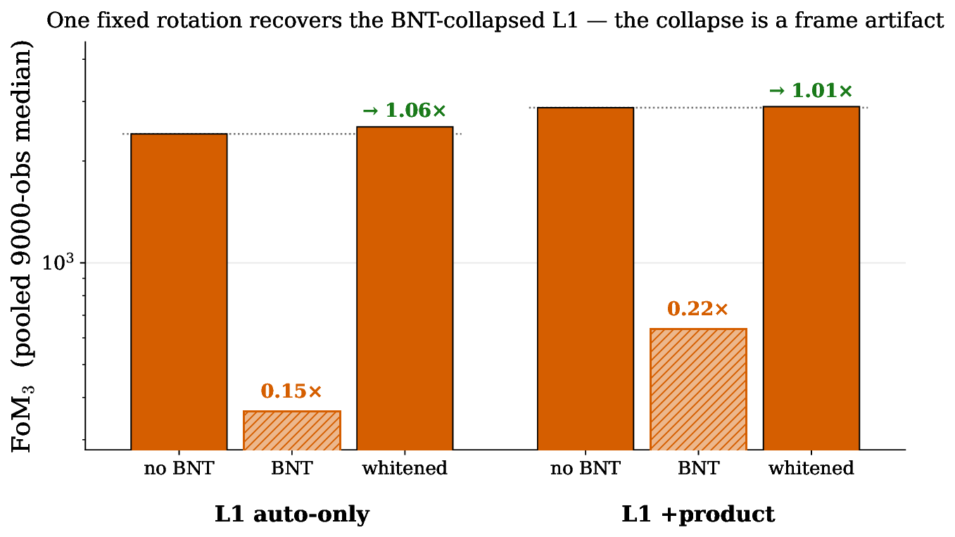
§2 The clincher: a frame artifact, not lost information (one rotation recovers ℓ1, 1.06×)

no-BNT, BNT collapsed, and whitened (recovered to 1.06x) per arm

the information was never lost

One fixed whitening rotation Q recovers the full no-BNT FoM3 for ℓ1 too (1.06×)
The collapse is a per-channel frame artifact: mix the bins, or re-rotate once
Confirms the intuition block; closes the Vinciguerra loop

Closes the Vinciguerra loop: their forecast said recovering the BNT SNR for HOS is "highly non-trivial"; here it is, in one fixed rotation. A frames result: a one-point statistic's information content is basis-dependent, and BNT is simply a poor frame for a per-channel statistic.

§3 One story: the optimal tomographic strategy (BNT becomes viable once the summary mixes bins)

per-bin l1 contours inflate under BNT — problem: the per-bin ℓ1 inflates under BNT

→

whitening recovers the l1 information — resolution: mix the bins, or re-rotate

one escalating story about cross-bin information

P(k) → ℓ1 (much more, even on safe scales) → learned (a bit more, calibrated)
Per-bin statistics cannot access cross-bin info (break under BNT); a channel-mixing compressor can (BNT-lossless)
BNT becomes viable once the summary mixes bins

Forward-looking: a route to baryon-robust, non-Gaussian SBI that keeps BNT's clean per-bin scale cuts without the contour-inflation tax. A next step, not a finished end-to-end measurement.