Impact of Weak Lensing Mass Mapping Algorithms on Cosmology Inference
January 16th, 2025
Andreas Tersenov



Le problème en question
- Weak lensing inference with higher-order statistics (HOS) often relies on mass maps.
- Producing these maps is an ill-posed inverse problem — there is no unique solution.
- Current surveys use simplistic algorithms because they are computationally efficient.
This raises an important question:
Does the choice of mass mapping algorithm affect the inferred cosmological parameters?
Or does it not matter, as long as the same operator is applied to both data and simulations?
How to test this properly?
We need to create a pipeline that can:

$\,$Introduction - Weak Lensing$\,$
- WL = Observational technique in cosmology for studying the matter distribution in the universe
- Principle: deflection of light from distant galaxies by gravitational fields → causes image distortion
- Weak → subtle & coherent distortions of background galaxy shapes
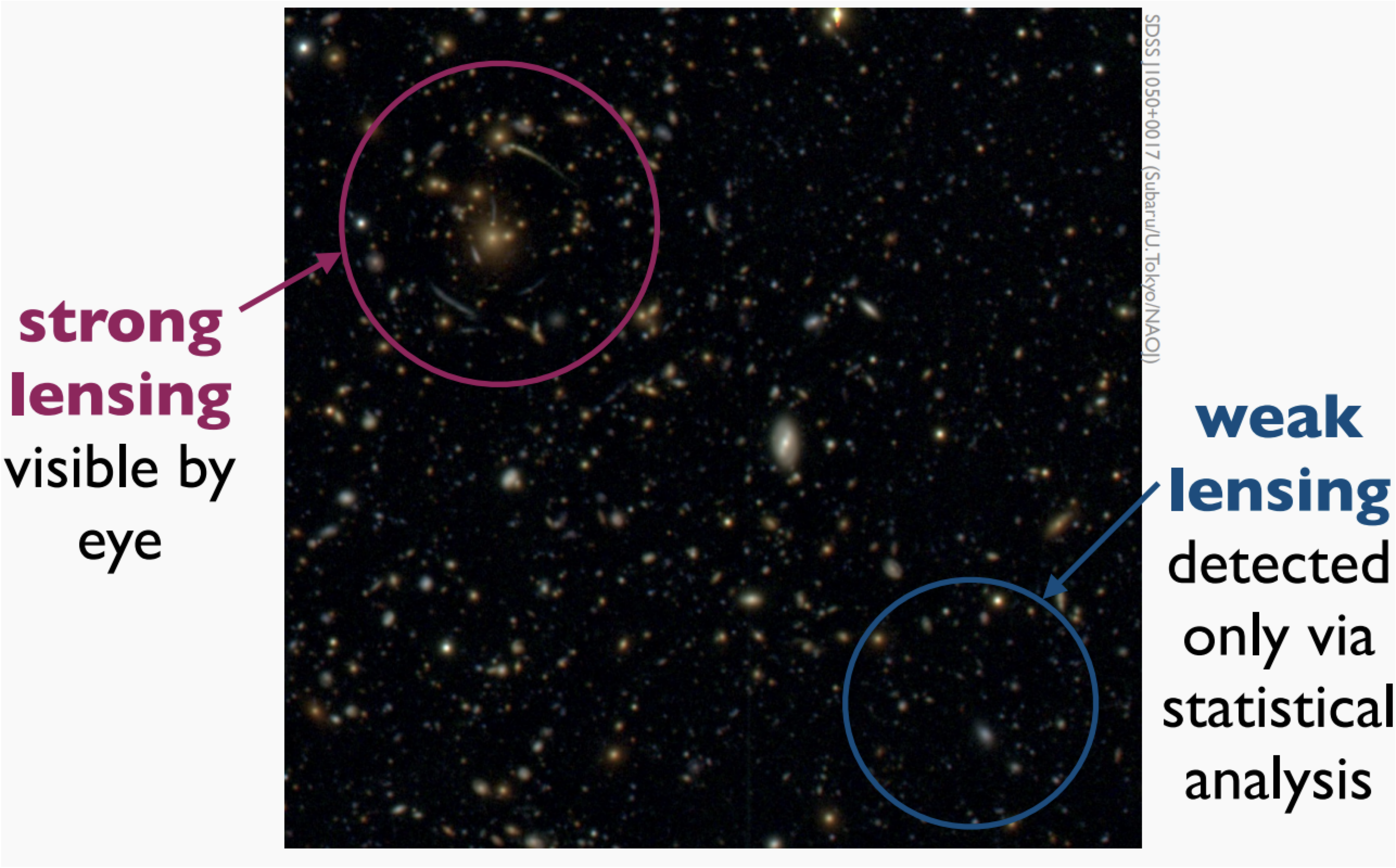
- WL provides a direct measurement of the gravitational distortion.
- WL enables us to probe the cosmic structure, investigate the nature of dark matter, and constrain cosmological parameters.
Shear & Convergence
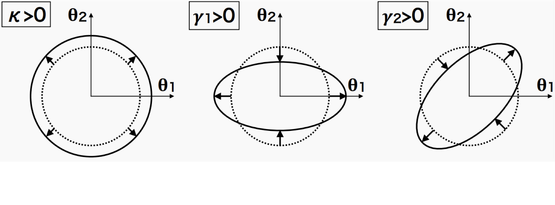
Convergence $\kappa$
$$ \kappa = \frac{1}{2} (\partial_1 \partial_1 + \partial_2 \partial_2) \psi =
\frac12
\nabla^2 \psi $$
⟶ difficult to measure
Shear $\gamma$
$$ \gamma_1 = \frac{1}{2} (\partial_1 \partial_1 - \partial_2 \partial_2) \psi,
\,\,
\gamma_2 = \partial_1 \partial_2 \psi $$
⟶ can be measured by statistical analysis of galaxy shapes
Shear estimation
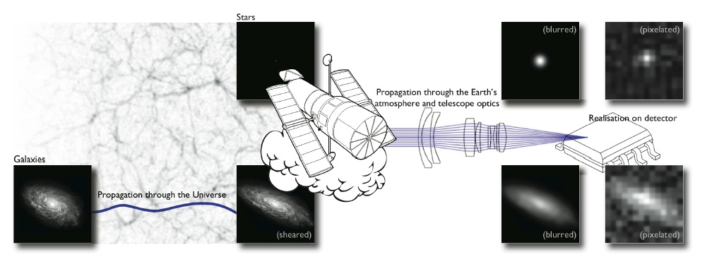
Galaxy shapes as estimators for gravitational shear
$$ e = \gamma + e_i \qquad \mbox{ with } \qquad e_i \sim \mathcal{N}(0, I)$$
- We are trying the measure the ellipticity $e$ of galaxies as an estimator for the gravitational shear $\gamma$
Advantages of Convergence
- Direct physical interpretation → $\kappa$: dimensionless measure of the surface mass density along LOS
- $\kappa$-map shows the LSS of the Universe → allows comparisons with other tracers of matter distribution
- Probes dark matter and its properties directly
- Easier to work with than shear: scalar quantity instead of spin-2 field
- Allows higher order statistics in a convenient way
- Cosmological parameter estimations → can be used to constrain cosmological parameters
Relation between $\kappa$ and $\gamma$
- From convergence to shear: $\,\, \gamma_i = \hat{P}_i \kappa$
- From shear to convergence: $\,\, \kappa = \hat{P}_1 \gamma_1 + \hat{P}_2 \gamma_2$
$$ \hat{P}_1(k)=\dfrac{k_1^2 - k_2^2}{k^2}, \,\,
\hat{P}_2(k)=\dfrac{2k_1k_2}{k^2} $$
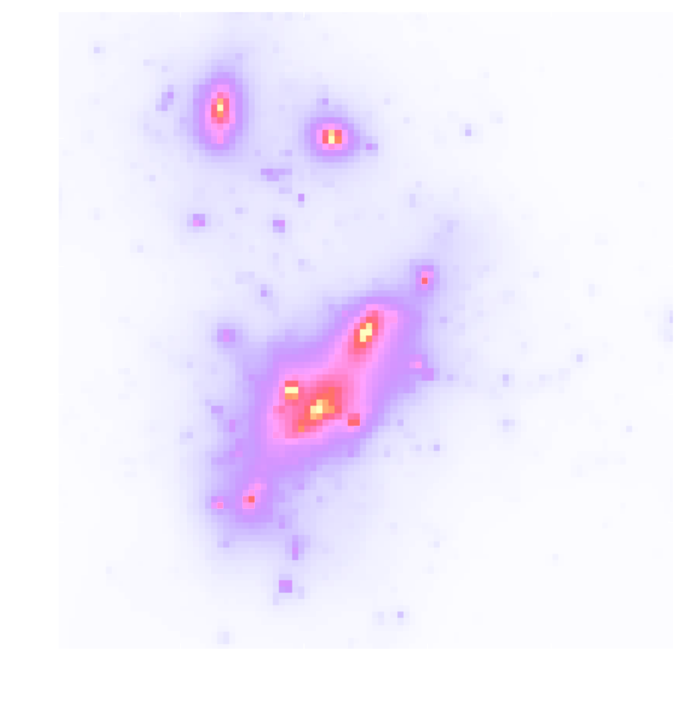
The Weak Lensing Mass-Mapping as an Inverse Problem
Shear $\gamma$
![]()
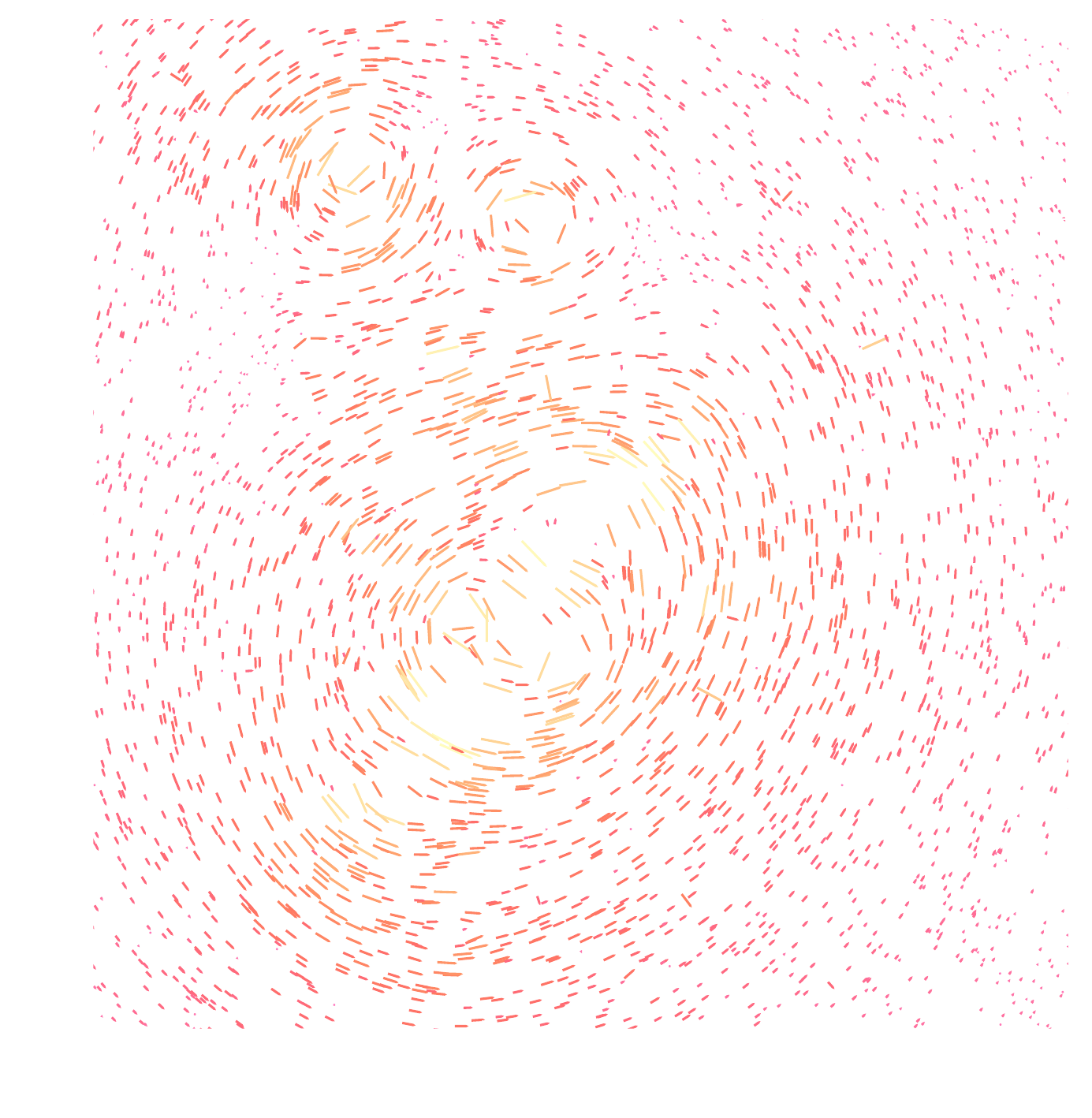
Convergence $\kappa$
![]()
$$\gamma_1 = \frac{1}{2} (\partial_1^2 - \partial_2^2) \ \Psi \quad;\quad \gamma_2 = \partial_1
\partial_2 \ \Psi \quad;\quad \kappa = \frac{1}{2} (\partial_1^2 + \partial_2^2) \ \Psi$$
$$\boxed{\gamma = \mathbf{P} \kappa}$$
Kaiser-Squires inversion
- Mass mapping problem recover an estimate of the convergence from measurements of the shear $$\kappa = \dfrac12 \Delta \psi, \,\, \gamma_1 = \dfrac12 \left( \partial_1^2 \psi - \partial_2^2 \psi \right), \,\, \gamma_2 = \partial_1 \partial_2 \psi $$ $$\Rightarrow \kappa = \Delta^{-1} \left[ \left( \partial_1^2 - \partial_2^2 \right) \gamma_1 + 2\partial_1 \partial_2 \gamma_2 \right] $$
Kaiser-Squires estimator:
$$ \tilde{\kappa}_E+i \tilde{\kappa}_B=\left(\frac{k_1^2-k_2^2}{k^2}+i \frac{2 k_1
k_2}{k^2}\right)\left(\tilde{\gamma}_1+i
\tilde{\gamma}_2\right)=\mathbf{P}\left(\tilde{\gamma}_1+i \tilde{\gamma}_2\right)
$$
→ $\tilde{\kappa}_E$ and $\tilde{\kappa}_B$ are complex representations of convergence E and B modes.
From galaxies to mass maps
Mass mapping as an inverse problem
- Binned data: $\gamma = F^* P F \, \kappa$
- Unbinned data: $\gamma = T^* P F \, \kappa$
$T =$ Non Equispaced Disctrete Fourier Transform (NDFT)
$$ \tilde{\boldsymbol{\kappa}}=\min _{\boldsymbol{\kappa}}\|\boldsymbol{\gamma}-\mathbf{A}
\boldsymbol{\kappa}\|_{\boldsymbol{\Sigma}_n}^2 $$
with $\mathbf{A} = \boldsymbol{F} \mathbf{P} \boldsymbol{F}^* $
There is no unique and stable solution, it is an ill-posed problem.
Mass Mapping
Kaiser-Squires inversion
Advantages:
- Simple linear operator
- Very easy to implement in Fourier space
- Optimal, in theory
Practical difficulties:
- Shear measurements are discrete, noisy, and irregularly sampled
- We actually measure the reduced shear: $g = \gamma/(1-\kappa)$
- Masks and integration over a subset of $\mathbb{R}^2$ lead to border errors ⇒ missing data problem
- Convergence is recoverable up to a constant ⇒ mass-sheet degeneracy problem
Inpainting
- Inpainting methods → techniques to fill in missing data in images by estimating the missing values from the known ones.
- A way to deal with the missing data problem in mass mapping and with the border effects in the convergence field.
- Implement a sparse inpainting based on the DCT (assume that the full $\kappa$-field is sparse in the DCT dictionary → apply an iterative thresholding algorithm to recover the missing data).
Bayesian reconstruction
- Mass mapping problem → statistical inference problem
- Goal: infer most probable value of $\kappa$-field given observed shear data
- Likelihood distribution: prob. of observing $\gamma$ data given true $\kappa$ → encodes the forward process of the model → contains the physics
- Prior distribution: encodes the knowledge about the signal before observing data
- Log-likelihood (when the noise is white Gaussian) $$\log p(\gamma \mid \kappa)=-\frac{1}{2}\left(\gamma-\mathbf{F}^* \mathbf{P F} \kappa\right)^{\dagger} \Sigma_n^{-1}\left(\gamma-\mathbf{F}^* \mathbf{P F} \kappa\right)+\text { constant }$$
- Maximum A Posteriori solution $$\hat{x} = \arg \max_x \, \log p(y|x) + \log p(x)$$
Wiener filter
- Assumes prior on $\kappa$ → Gaussian random field $p_{\rm Gauss}(\kappa) = \frac{1}{\sqrt{\det 2\pi \mathbf{S}}} \exp{\left( - \frac12 \tilde{\kappa}^{\dagger} \mathbf{S}^{-1} \tilde{\kappa} \right)}$
- Likelihood (assuming uncorrelated, Gaussian noise) → also Gaussian $p(\mathbf{\gamma} | \kappa) = \frac{1}{\sqrt{2\pi\det \mathbf{N}}} \exp{\left[ -\frac12 (\mathbf{\gamma - \mathbf{A} \mathbf{\kappa}})^{\dagger} \mathbf{N}^{-1} ( \gamma - \mathbf{A} \mathbf{\kappa} ) \right]}$
- The Gaussian prior encodes the assumption that the fluctuations in the $\kappa$-field are well described by a Gaussian random field, with power spectrum given by the cosmological model
Convergence power spectrum
$$ \langle \tilde{\kappa}(\boldsymbol{k}) \tilde{\kappa}^*(\boldsymbol{k}') \rangle =
(2\pi)^2
\delta_D(\boldsymbol{k} - \boldsymbol{k}') P_{\kappa}(k) $$
Stat. measure of the spatial distribution of the convergence field → quantifies the
amplitude of the fluctuations in κ as function of their spatial scale
Wiener filter
Wiener solution of the inverse problem
$$\hat{\kappa}_{\text {wiener }}=\arg \min _\kappa\left\|\Sigma^{-1 /
2}\left(\gamma-\mathbf{F}^* \mathbf{P F} \kappa\right)\right\|_2^2+\log p_{\text {Gaussian
}}(\kappa)$$
- This solution corresponds to the maximum a posteriori (MAP) solution under the assumption of a Gaussian prior on $\kappa$, and it matches the mean of the Gaussian posterior.
Wiener reconstruction
$$\hat{\kappa}_{\text {wiener }}=\mathbf{S} \mathbf{P}^{\dagger}
\left[\mathbf{P} \mathbf{S} \mathbf{P}^{\dagger} + \mathbf{N} \right]^{-1} \tilde{\gamma}$$
Sparse recovery
- Decomposes the signal into another domain (dictionary), where it is sparse
- Implement the wavelet transform → decomposes the signal into wavelet functions (waveforms of limited duration with an average value of zero)
- Use starlet wavelets → represent well structures resembling the $\kappa$ of a DM halo (positive & isotropic)
- The application of sparsity prior enforces a cosmological model where the matter field is a combination of spherically symmetric DM halos
MCALens
- Models $\kappa$-field as a sum of a Gaussian and non-Gaussian component $$\boxed{\kappa = \underbrace{\kappa_{\rm NG}}_{\text{Standard Wiener filter approach}} + \underbrace{\kappa_\rm G}_{\text{Modified wavelet approach}}}$$ $$\min _{\kappa_G, \kappa_{N G}}\left\|\gamma-\mathbf{A}\left(\kappa_G+\kappa_{N G}\right)\right\|_{\Sigma_n}^2+C_{\mathrm{G}}\left(\kappa_G\right)+C_{\mathrm{NG}}\left(\kappa_{N G}\right) $$
- MCA (morphological Component Analysis) performs an alternating
minimization
scheme:
- Estimate $\mathbf{\kappa}_{\mathrm{G}}$ assuming $\mathbf{\kappa}_{\mathrm{NG}}$ is known: $$\min _{\kappa_G}\left\|\left(\gamma-\mathbf{A}\kappa_{N G}\right) -\mathbf{A}\kappa_{G} \right\|_{\Sigma_n}^2+C_{\mathrm{G}}\left(\kappa_G\right)$$
- Estimate $\mathbf{\kappa}_{\mathrm{NG}}$ assuming $\mathbf{\kappa}_{\mathrm{G}}$ is known: $$\min _{\kappa_{NG}}\left\|\left(\gamma-\mathbf{A}\kappa_{G}\right) -\mathbf{A}\kappa_{NG} \right\|_{\Sigma_n}^2+C_{\mathrm{NG}}\left(\kappa_{NG}\right)$$
Overview of mass mapping methods
- Wiener filter: Prior on $\kappa$ → Gaussian random field, Likelihood → Gaussian, Solution → corresponds to MAP for gaussian $\kappa$
- Sparse recovery: Prior on $\kappa$ → sparse in wavelet basis, Enforces model where matter field is a combination of DM halos
- MCALens: Models $\kappa$-field as sum of a Gaussian and a non-Gaussian component, Uses Morphological Component Analysis
- Deep Learning Methods:
- DeepMass: CNN with a U-Net-based architecture, prior from simulations
- DeepPosterior: Probabilistic mass mapping with deep generative models, Prior from 2pt statistics modelling at large scales & Deep Learning on simulations for small scales, Sampling with Annealed HMC
Mass mapping methods:
\[
\begin{array}{ll}
\hline \hline
\text{Method} & \text{RMSE} \downarrow \\
\hline
\text{KS } & 1.1 \times 10^{-2} \\
\text{iKS } & 1.1 \times 10^{-2} \\
\text{MCALens} & 9.8 \times 10^{-3} \\
\hline
\end{array}
\]
Statistics
Higher Order Statistics: Peak Counts
- Peaks: local maxima of the SNR field $\nu = \dfrac{\left(\mathcal{W} \ast \kappa \right)(\theta_{\rm ker})}{\sigma_n^{\rm filt}}$
- Peaks trace regions where the value of $\kappa$ is high → they are associated to massive structures
Peak funtions
- The peak function is the number of peaks in a map as a function of the SNR $\nu$
Wavelet peaks
- We consider a multi-scale analysis compared to a single-scale analysis
- Apply (instead of Gaussian filter) a starlet transform → allows us to represent an image $I$ as a sum of wavelet coefficient images and a coarse resolution image
- Allows for the simultaneous processing of data at different scales → efficiency
- Each wavelet band covers a different frequency range, which leads to an almost diagonal peak count covariance matrix
Wavelet peak funtions
What happens if we consider all pixels instead of selecting multi-scale minima and maxima?
Starlet $\ell_1$-norm
- New higher order summary statistic for weak lensing observables
- Provides a fast multi-scale calculation of the full void and peak distribution
- $\ell_1$-norm = sum of absolute values of the starlet decomposition coefficients of a weak lensing map
- Information encoded in all pixels
- Automatically includes peaks and voids
- Multi-scale approach
- Avoids the problem of defining peaks and voids
Inference
Inference with HOS
- Use $\texttt{cosmoSLICS}$ simulations: suite designed for the analysis of WL data beyond the standard 2pt cosmic shear
- $\texttt{cosmoSLICS}$ cover a wide parameter space in $\left[ \Omega_m, \sigma_8, w_0, h \right]$.
- For Bayesian inference → use a Gaussian likelihood for a cosmology independent covariance, and a flat prior.
- To have a prediction of each HOS given a new set of parameters→ employ an interpolation with Gaussian Process Regressor (GPR)
Noise & Covariance
- We consider Gaussian, but non-white noise → the noise depends on the number of galaxies in each pixel $$\sigma_n = \dfrac{\sigma_{\epsilon}}{\sqrt{2 n_{\rm gal} A_{\rm pix}}}$$
- We incorporate masks
- Calculate covariance: $$ \boxed{C_{ij} = \sum_{r=1}^N \dfrac{\left( x_i^r - \mu_i \right) \left( x_j^r - \mu_j \right)}{N-1}} \, , \,\,\,\mu_i = \dfrac{1}{N} \sum_r x_i^r $$
From data to contours
- $\mu$: expected theoretical prediction, $d$: data array (mean over realizations of a HOS), $C$: covariance matrix
So does the choice of the mass mapping algorithm matter for the final constraints?
The (standard) mono-scale peak counts
\[
\begin{array}{lcccc}
\hline \hline
\text{FoM} & \text{KS} & \text{iKS} & \text{MCALens} \\
\hline \hline
\left(\Omega_m, h\right) & 476 & 453 & 450 \\
\left(\Omega_m, w_0\right) & 152 & 141 & 233 \\
\left(\Omega_m, \sigma_8\right) & 1323 & 1285 & 1740 \\
\left(h, w_0\right) & 55 & 63 & 87 \\
\left(h, \sigma_8\right) & 336 & 292 & 293 \\
\left(w_0, \sigma_8\right) & 75 & 72 & 124 \\
\hline
\left(\Omega_m, h, w_0, \sigma_8\right) & 492 & 444 & 578 \\
\hline
\end{array}
\]
Wavelet multi-scale peak counts
\[
\begin{array}{lcccc}
\hline \hline
\text{FoM} & \text{KS} & \text{iKS} & \text{MCALens} \\
\hline \hline
\left(\Omega_m, h\right) & 670 & 702 & 2159 \\
\left(\Omega_m, w_0\right) & 247 & 244 & 1051 \\
\left(\Omega_m, \sigma_8\right) & 2414 & 2517 & 9039 \\
\left(h, w_0\right) & 82 & 80 & 259 \\
\left(h, \sigma_8\right) & 411 & 433 & 1335 \\
\left(w_0, \sigma_8\right) & 131 & 129 & 577 \\
\hline
\left(\Omega_m, h, w_0, \sigma_8\right) & 758 & 755 & 1947 \\
\hline
\end{array}
\]
Where does this improvement come from?
Conclusions
- Investigated how different mass mapping algorithms affect cosmological inference using HOS from WL data.
- Estimated posterior distributions of $\Omega_\mathrm{m}$, $\sigma_8$, $h$, and $w_0$ using peak counts and wavelet peak counts.
Results
- MCALens Advantage:
- $\sim 17\%$ improvement in (FoM) over KS.
- $\sim 157\%$ improvement in FoM over KS.
- KS vs. iKS: No significant difference in constraints → inpainting does not improve performance
- Wavelet Peak Counts: Provide tighter constraints than single-scale peak counts.
- MCALens and Multi-Scale Approach: Captures more small-scale information, leading to the greatest improvement.
Takeaway
- Careful Selection Matters: Choosing an advanced mass mapping method significantly enhances constraints on cosmological parameters from HOS.