Impact of mass mapping for cosmological parameter estimation
UNIONS meeting in Paris, June 24th, 2024
Andreas Tersenov
General Idea
Create a pipeline:
- Use it to investigate the impact of mass mapping algorithms on cosmology constraints.
- Use it on UNIONS/CFIS data to get observational constraints on cosmology.
- Use it to test novel mass mapping methods
Shear & Convergence
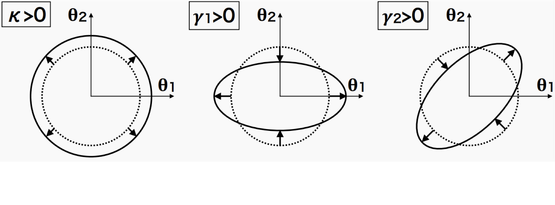
Convergence $\kappa$
$$ \kappa = \frac{1}{2} (\partial_1 \partial_1 + \partial_2 \partial_2) \psi =
\frac12
\nabla^2 \psi $$
⟶ difficult to measure
Shear $\gamma$
$$ \gamma_1 = \frac{1}{2} (\partial_1 \partial_1 - \partial_2 \partial_2) \psi,
\,\,
\gamma_2 = \partial_1 \partial_2 \psi $$
⟶ can be measured by statistical analysis of galaxy shapes
Shear estimation
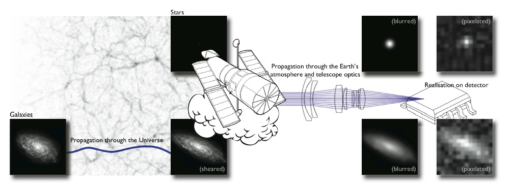
Galaxy shapes as estimators for gravitational shear
$$ e = \gamma + e_i \qquad \mbox{ with } \qquad e_i \sim \mathcal{N}(0, I)$$
- We are trying the measure the ellipticity $e$ of galaxies as an estimator for the gravitational shear $\gamma$
Advantages of Convergence
- Direct physical interpretation → $\kappa$: dimensionless measure of the surface mass density along LOS
- $\kappa$-map shows the LSS of the Universe → allows comparisons with other tracers of matter distribution
- Probes dark matter and its properties directly
- Easier to work with than shear: scalar quantity instead of spin-2 field
- Allows higher order statistics in a convenient way
- Cosmological parameter estimations → can be used to constrain cosmological parameters
Relation between $\kappa$ and $\gamma$
- From convergence to shear: $\,\, \gamma_i = \hat{P}_i \kappa$
- From shear to convergence: $\,\, \kappa = \hat{P}_1 \gamma_1 + \hat{P}_2 \gamma_2$
$$ \hat{P}_1(k)=\dfrac{k_1^2 - k_2^2}{k^2}, \,\,
\hat{P}_2(k)=\dfrac{2k_1k_2}{k^2} $$
The Weak Lensing Mass-Mapping as an Inverse Problem
Shear $\gamma$
![]()
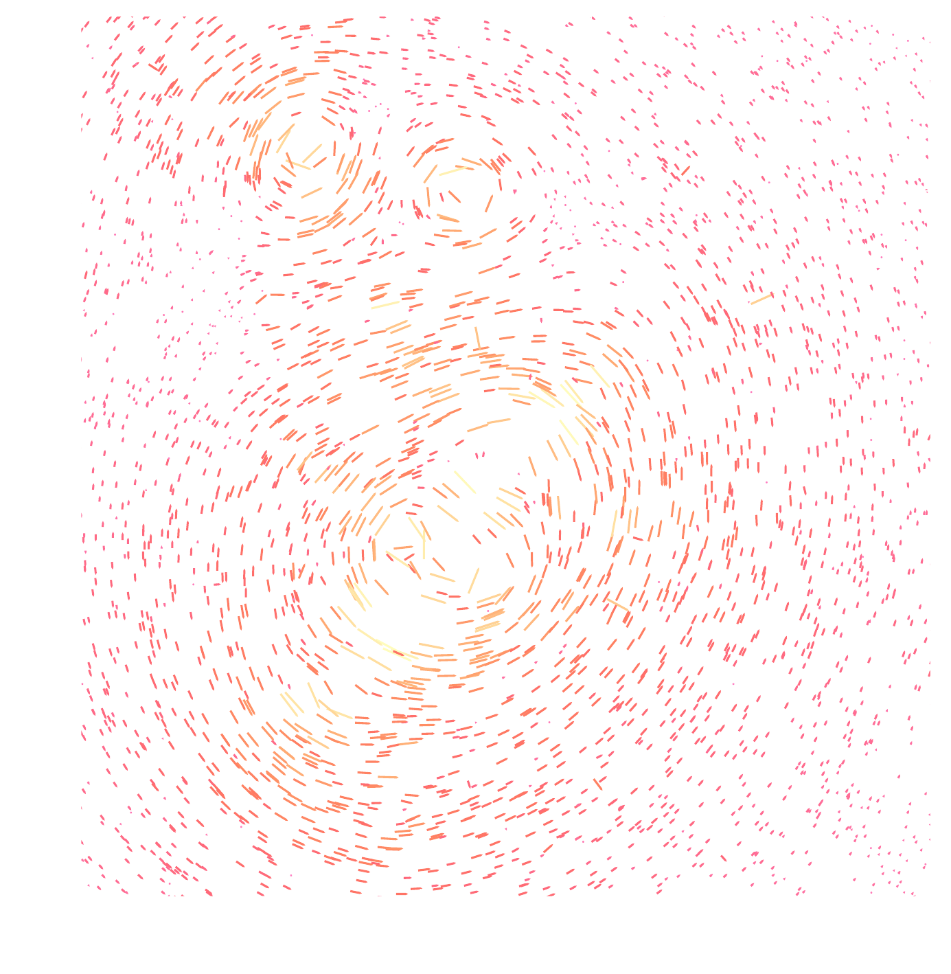
Convergence $\kappa$
![]()
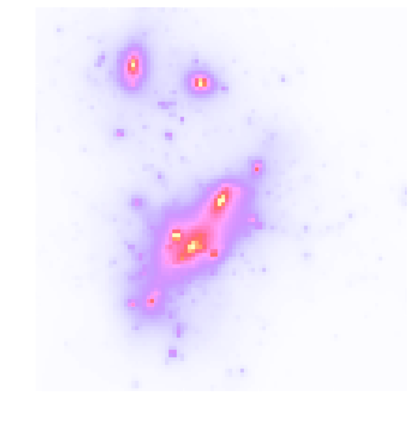
$$\gamma_1 = \frac{1}{2} (\partial_1^2 - \partial_2^2) \ \Psi \quad;\quad \gamma_2 = \partial_1
\partial_2 \ \Psi \quad;\quad \kappa = \frac{1}{2} (\partial_1^2 + \partial_2^2) \ \Psi$$
$$\boxed{\gamma = \mathbf{P} \kappa}$$
Kaiser-Squires inversion
- Mass mapping problem recover an estimate of the convergence from measurements of the shear $$\kappa = \dfrac12 \Delta \psi, \,\, \gamma_1 = \dfrac12 \left( \partial_1^2 \psi - \partial_2^2 \psi \right), \,\, \gamma_2 = \partial_1 \partial_2 \psi $$ $$\Rightarrow \kappa = \Delta^{-1} \left[ \left( \partial_1^2 - \partial_2^2 \right) \gamma_1 + 2\partial_1 \partial_2 \gamma_2 \right] $$
Kaiser-Squires estimator:
$$ \tilde{\kappa}_E+i \tilde{\kappa}_B=\left(\frac{k_1^2-k_2^2}{k^2}+i \frac{2 k_1
k_2}{k^2}\right)\left(\tilde{\gamma}_1+i
\tilde{\gamma}_2\right)=\mathbf{P}\left(\tilde{\gamma}_1+i \tilde{\gamma}_2\right)
$$
→ $\tilde{\kappa}_E$ and $\tilde{\kappa}_B$ are complex representations of convergence E and B modes.
From galaxies to mass maps
Mass mapping as an inverse problem
- Binned data: $\gamma = F^* P F \, \kappa$
- Unbinned data: $\gamma = T^* P F \, \kappa$
$T =$ Non Equispaced Disctrete Fourier Transform (NDFT)
$$ \tilde{\boldsymbol{\kappa}}=\min _{\boldsymbol{\kappa}}\|\boldsymbol{\gamma}-\mathbf{A}
\boldsymbol{\kappa}\|_{\boldsymbol{\Sigma}_n}^2 $$
with $\mathbf{A} = \boldsymbol{F} \mathbf{P} \boldsymbol{F}^* $
There is no unique and stable solution, it is an ill-posed problem.
Kaiser-Squires inversion
Advantages:
- Simple linear operator
- Very easy to implement in Fourier space
- Optimal, in theory
Practical difficulties:
- Shear measurements are discrete, noisy, and irregularly sampled
- We actually measure the reduced shear: $g = \gamma/(1-\kappa)$
- Masks and integration over a subset of $\mathbb{R}^2$ lead to border errors ⇒ missing data problem
- Convergence is recoverable up to a constant ⇒ mass-sheet degeneracy problem
Bayesian reconstruction
- Mass mapping problem → statistical inference problem
- Goal: infer most probable value of $\kappa$-field given observed shear data
- Likelihood distribution: prob. of observing $\gamma$ data given true $\kappa$ → encodes the forward process of the model → contains the physics
- Prior distribution: encodes the knowledge about the signal before observing data
- Log-likelihood (when the noise is white Gaussian) $$\log p(\gamma \mid \kappa)=-\frac{1}{2}\left(\gamma-\mathbf{F}^* \mathbf{P F} \kappa\right)^{\dagger} \Sigma_n^{-1}\left(\gamma-\mathbf{F}^* \mathbf{P F} \kappa\right)+\text { constant }$$
- Maximum A Posteriori solution $$\hat{x} = \arg \max_x \, \log p(y|x) + \log p(x)$$
Wiener filter
- Assumes prior on $\kappa$ → Gaussian random field $p_{\rm Gauss}(\kappa) = \frac{1}{\sqrt{\det 2\pi \mathbf{S}}} \exp{\left( - \frac12 \tilde{\kappa}^{\dagger} \mathbf{S}^{-1} \tilde{\kappa} \right)}$
- Likelihood (assuming uncorrelated, Gaussian noise) → also Gaussian $p(\mathbf{\gamma} | \kappa) = \frac{1}{\sqrt{2\pi\det \mathbf{N}}} \exp{\left[ -\frac12 (\mathbf{\gamma - \mathbf{A} \mathbf{\kappa}})^{\dagger} \mathbf{N}^{-1} ( \gamma - \mathbf{A} \mathbf{\kappa} ) \right]}$
- The Gaussian prior encodes the assumption that the fluctuations in the $\kappa$-field are well described by a Gaussian random field, with power spectrum given by the cosmological model
Convergence power spectrum
$$ \langle \tilde{\kappa}(\boldsymbol{k}) \tilde{\kappa}^*(\boldsymbol{k}') \rangle =
(2\pi)^2
\delta_D(\boldsymbol{k} - \boldsymbol{k}') P_{\kappa}(k) $$
Stat. measure of the spatial distribution of the convergence field → quantifies the
amplitude of the fluctuations in κ as function of their spatial scale
Wiener filter
Wiener solution of the inverse problem
$$\hat{\kappa}_{\text {wiener }}=\arg \min _\kappa\left\|\Sigma^{-1 /
2}\left(\gamma-\mathbf{F}^* \mathbf{P F} \kappa\right)\right\|_2^2+\log p_{\text {Gaussian
}}(\kappa)$$
- This solution corresponds to the maximum a posteriori (MAP) solution under the assumption of a Gaussian prior on $\kappa$, and it matches the mean of the Gaussian posterior.
Wiener reconstruction
$$\hat{\kappa}_{\text {wiener }}=\mathbf{S} \mathbf{P}^{\dagger}
\left[\mathbf{P} \mathbf{S} \mathbf{P}^{\dagger} + \mathbf{N} \right]^{-1} \tilde{\gamma}$$
Sparse recovery
- Decomposes the signal into another domain (dictionary), where it is sparse
- Implement the wavelet transform → decomposes the signal into wavelet functions (waveforms of limited duration with an average value of zero)
- Use starlet wavelets → represent well structures resembling the $\kappa$ of a DM halo (positive & isotropic)
- The application of sparsity prior enforces a cosmological model where the matter field is a combination of spherically symmetric DM halos
MCALens
- Models $\kappa$-field as a sum of a Gaussian and non-Gaussian component $$\boxed{\kappa = \underbrace{\kappa_{\rm NG}}_{\text{Standard Wiener filter approach}} + \underbrace{\kappa_\rm G}_{\text{Modified wavelet approach}}}$$ $$\min _{\kappa_G, \kappa_{N G}}\left\|\gamma-\mathbf{A}\left(\kappa_G+\kappa_{N G}\right)\right\|_{\Sigma_n}^2+C_{\mathrm{G}}\left(\kappa_G\right)+C_{\mathrm{NG}}\left(\kappa_{N G}\right) $$
- MCA (morphological Component Analysis) performs an alternating
minimization
scheme:
- Estimate $\mathbf{\kappa}_{\mathrm{G}}$ assuming $\mathbf{\kappa}_{\mathrm{NG}}$ is known: $$\min _{\kappa_G}\left\|\left(\gamma-\mathbf{A}\kappa_{N G}\right) -\mathbf{A}\kappa_{G} \right\|_{\Sigma_n}^2+C_{\mathrm{G}}\left(\kappa_G\right)$$
- Estimate $\mathbf{\kappa}_{\mathrm{NG}}$ assuming $\mathbf{\kappa}_{\mathrm{G}}$ is known: $$\min _{\kappa_{NG}}\left\|\left(\gamma-\mathbf{A}\kappa_{G}\right) -\mathbf{A}\kappa_{NG} \right\|_{\Sigma_n}^2+C_{\mathrm{NG}}\left(\kappa_{NG}\right)$$
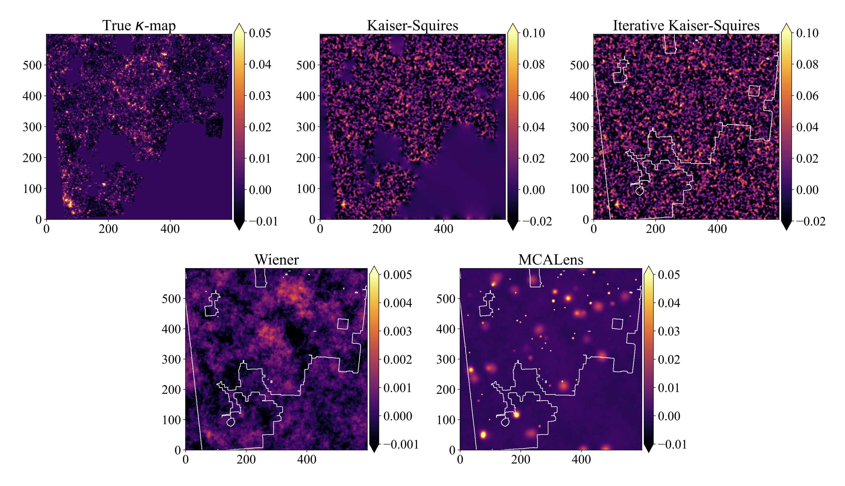
Overview of mass mapping methods
- Wiener filter: Prior on $\kappa$ → Gaussian random field, Likelihood → Gaussian, Solution → corresponds to MAP for gaussian $\kappa$
- Sparse recovery: Prior on $\kappa$ → sparse in wavelet basis, Enforces model where matter field is a combination of DM halos
- MCALens: Models $\kappa$-field as sum of a Gaussian and a non-Gaussian component, Uses Morphological Component Analysis
- Deep Learning Methods:
- DeepMass: CNN with a U-Net-based architecture, prior from simulations
- DeepPosterior: Probabilistic mass mapping with deep generative models, Prior from 2pt statistics modelling at large scales & Deep Learning on simulations for small scales, Sampling with Annealed HMC
Mass mapping methods:
Higher Order Statistics: Peak Counts
- Peaks: local maxima of the SNR field $\nu = \dfrac{\left(\mathcal{W} \ast \kappa \right)(\theta_{\rm ker})}{\sigma_n^{\rm filt}}$
- Peaks trace regions where the value of $\kappa$ is high → they are associated to massive structures
Wavelet peaks
- We consider a multi-scale analysis compared to a single-scale analysis
- Apply (instead of Gaussian filter) a starlet transform → allows us to represent an image $I$ as a sum of wavelet coefficient images and a coarse resolution image
- Allows for the simultaneous processing of data at different scales → efficiency
- Each wavelet band covers a different frequency range, which leads to an almost diagonal peak count covariance matrix
What happens if we consider all pixels instead of selecting multi-scale minima and maxima?
Starlet $\ell_1$-norm
- New higher order summary statistic for weak lensing observables
- Provides a fast multi-scale calculation of the full void and peak distribution
- $\ell_1$-norm = sum of absolute values of the starlet decomposition coefficients of a weak lensing map
- Information encoded in all pixels
- Automatically includes peaks and voids
- Multi-scale approach
- Avoids the problem of defining peaks and voids
Simulations
- Use $\texttt{cosmoSLICS}$ simulations: suite designed for the analysis of WL data beyond the standard 2pt cosmic shear, mimicking the DES Y1 data.
- $\texttt{cosmoSLICS}$ sample wide volume in
$\left[ \Omega_m, \sigma_8, w_0, h \right]$ with 25 points aranged into a
Latin hypercube.
- The output of each simulation includes a galaxy catalogue of $10\times 10 \, \rm deg^2$ with positions, $\epsilon$, $\gamma$, $\kappa$, $z$, and metacal weights that match those of the real data.
- The covariance matrix that captures the sample variance is estimated from 124 fully independent $\texttt{SLICS}$ N-body simulations.
- These are evolved from independent initial conditions at a fixed cosmology.
- We increase the effective number of covariance mocks by randomly shuffling 10 times the shear components and generating different realizations of the noise field.
Noise & Covariance
- We consider Gaussian, but non-white noise → the noise depends on the number of galaxies in each pixel $$\sigma_n = \dfrac{\sigma_{\epsilon}}{\sqrt{2 n_{\rm gal} A_{\rm pix}}}$$
- We incorporate masks
- Calculate covariance: $$ \boxed{C_{ij} = \sum_{r=1}^N \dfrac{\left( x_i^r - \mu_i \right) \left( x_j^r - \mu_j \right)}{N-1}} \, , \,\,\,\mu_i = \dfrac{1}{N} \sum_r x_i^r $$
Starlet filter tends to make the covariance matrix more diagonal
Inference
- For Bayesian inference → use a Gaussian likelihood for a cosmology independent covariance, and a flat prior. $$ \log \mathcal{L} = -\dfrac12 \left[ d - \mu(\theta) \right]^T C^{-1} \left[ d - \mu(\theta) \right]$$
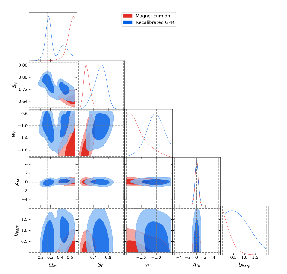
- To have a prediction of each HOS given a new set of parameters→ employ an interpolation with Gaussian Process Regressor (GPR) → issues (parameter space is too sparse, and sometimes the GPR is not able to interpolate well, introducing artefacts in the prediction).
- At the moment we are also exploring the use of neural networks for our emulator.
From data to contours
- $\mu$: expected theoretical prediction, $d$: data array (mean over realizations of a HOS), $C$: covariance matrix
So does the choice of the mass mapping algorithm matter for the final constraints?
The (standard) mono-scale peak counts
Wavelet multi-scale peak counts
From Harnois-Deraps et al (2024) paper
Conclusions
- Mass mapping is a challenging problem in weak lensing
- Several methods have been developed, each with its advantages and limitations
- HOS provide complementary information to the standard 2pt statistics, and can help extract more information from the data & break degeneracies
Results
- Created pipeline for HOS analysis of weak lensing catalogs
- Implemented it to show that the choice of the mass mapping algorithm has a significant impact on the cosmological constraints
Future work
- Add DL methods to the pipeline
- Use the pipeline for a HOS analysis of UNIONS data
- Develop PnP mass mapping method