Higher-order weak lensing, COSMO-26 Leiden

COSMO-26, Leiden, 24–28 August 2026

Unlocking Non-Gaussian Information in Weak Lensing

Baryonic robustness, and analytical vs learned summaries

Andreas Tersenov FORTH, U. Crete, CEA Paris-Saclay

with Sacha Guerrini, Jean-Luc Starck and Martin Kilbinger
slides: https://andreastersenov.github.io/talks/cosmo26/

The non-Gaussian information and the worst small-scale systematic live on the same scales

To be able to trust our HOS results we must investigate how they are affected by each systematic at the contour level.

question 1

How much does unmodelled feedback bias our higher-order statistics, and how does that grow with survey area?

question 2

Once those scales are cut, is there any constraining power left to gain over the power spectrum?

SAY: higher-order statistics are usually demonstrated on clean simulations; Stage IV is systematics-limited, so what decides whether we can use them is how they behave under contamination. Baryonic feedback - AGN and supernovae - pushes gas out of haloes and suppresses matter on small scales, mimicking a cosmological signal, exactly where the constraining power lives and where the feedback models disagree most with each other. Point at the figure and let the room read it before any band appears: both the extra information and the contamination live at small scales. Now, the conservative response is to throw the affected scales away. The question is how much that costs. CLICK - OPTIMISTIC: only the smallest scales are affected, we cut them, and most of the non-Gaussian information is still there. CLICK - PESSIMISTIC: the contamination reaches much further, and once you cut it there is nothing beyond-Gaussian left worth having - the power spectrum would do just as well. Which of these is true is an empirical question, and it is the first thing we measured.

§1 Wavelet peak counts and the $\ell_1$-norm are 1-pt statistics on the same starlet decomposition

the starlet transform: a convergence map written as the sum of four wavelet-coefficient bands plus a coarse map, each band carrying structure of a characteristic angular size — the **starlet transform**: one map as a sum of band-pass images, each carrying structure of a characteristic angular size

wavelet peak counts

a smoothed convergence map with its signal-to-noise peaks circled

local maxima of the SNR field, counted per SNR bin → focus only on a subset of the field

starlet ℓ1-norm

$$\ell_1^{\,j,i} \;=\; \sum_{u=1}^{\#\mathcal{S}_{j,i}} \big| \mathcal{S}_{j,i}[u] \big| \;=\; \lVert \mathcal{S}_{j,i} \rVert_1$$

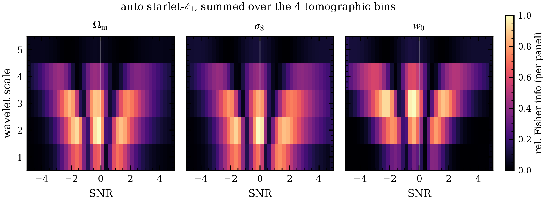
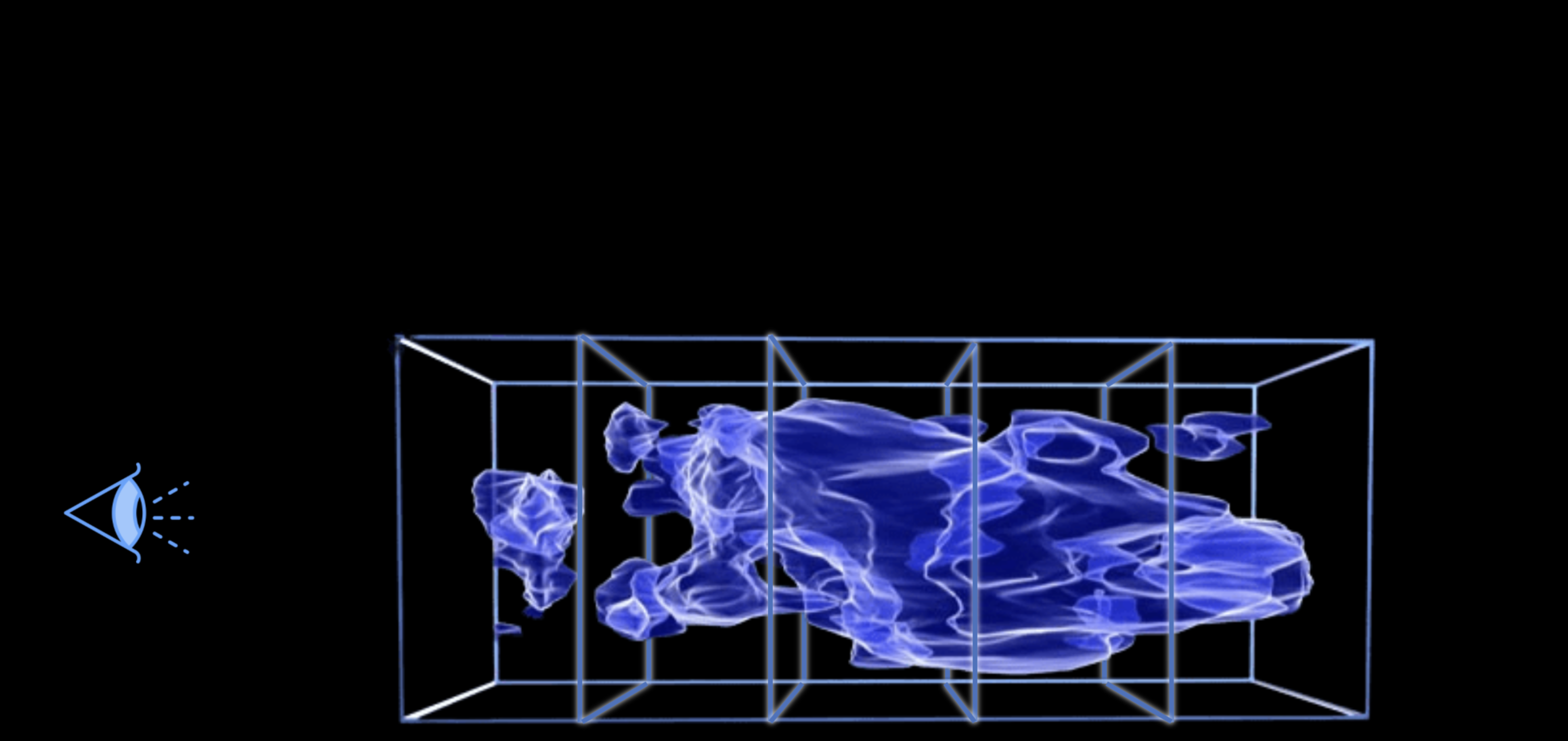
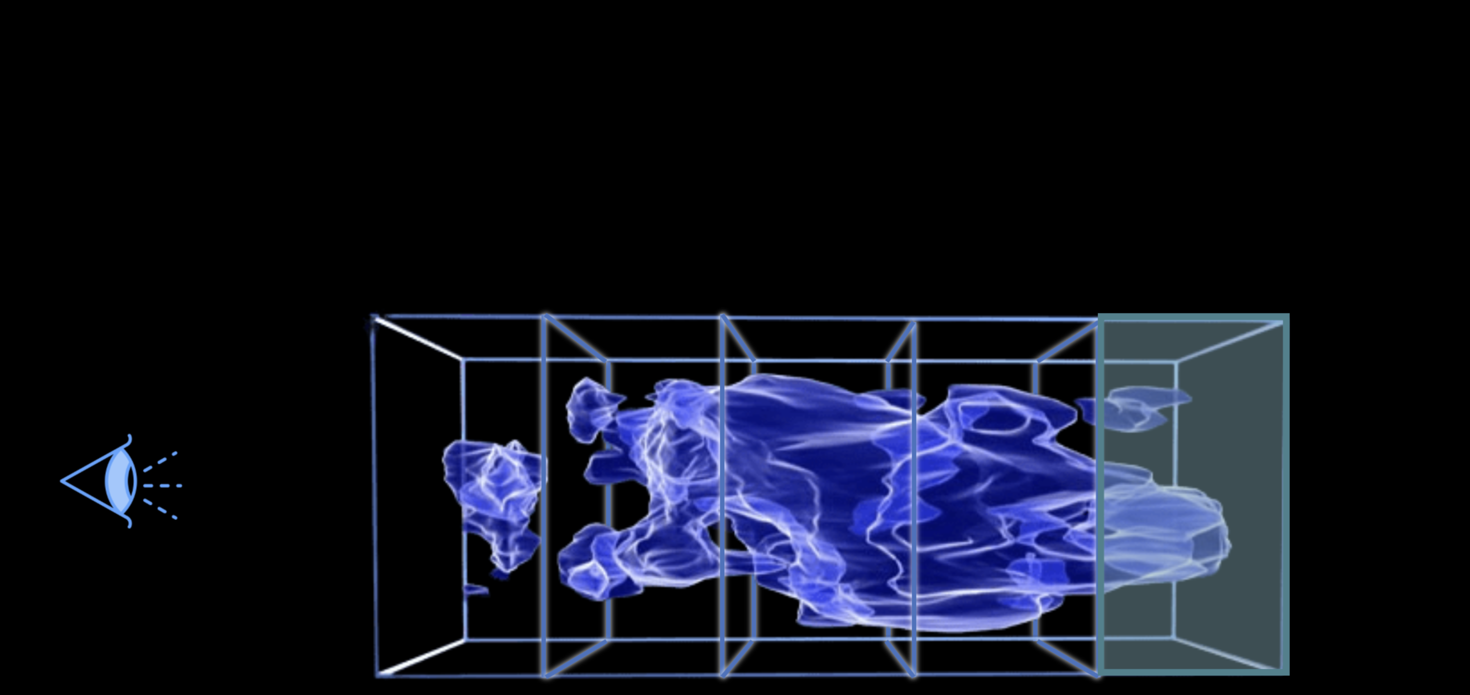
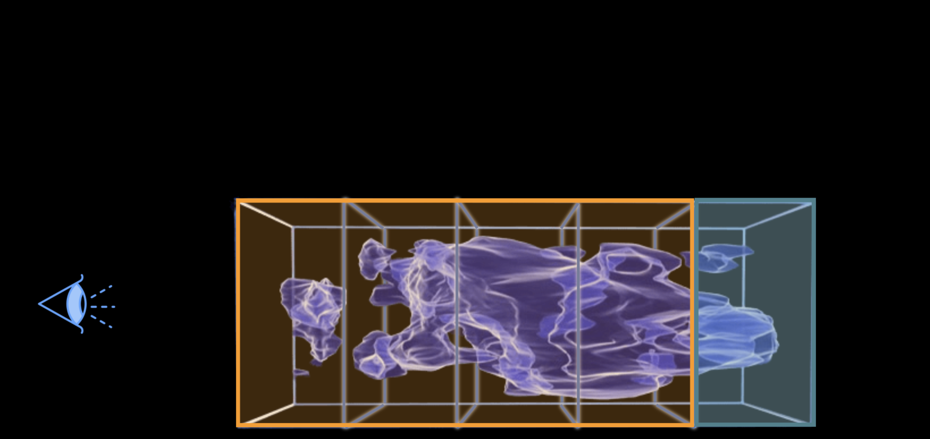
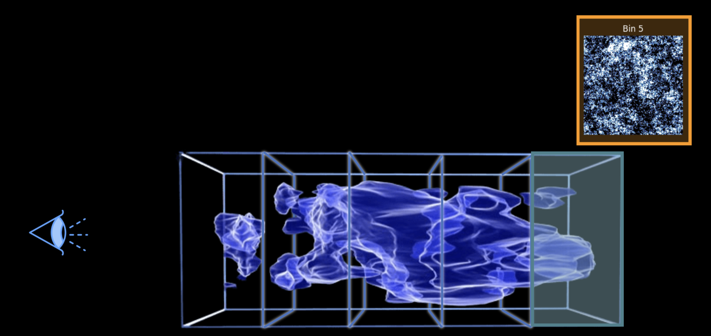
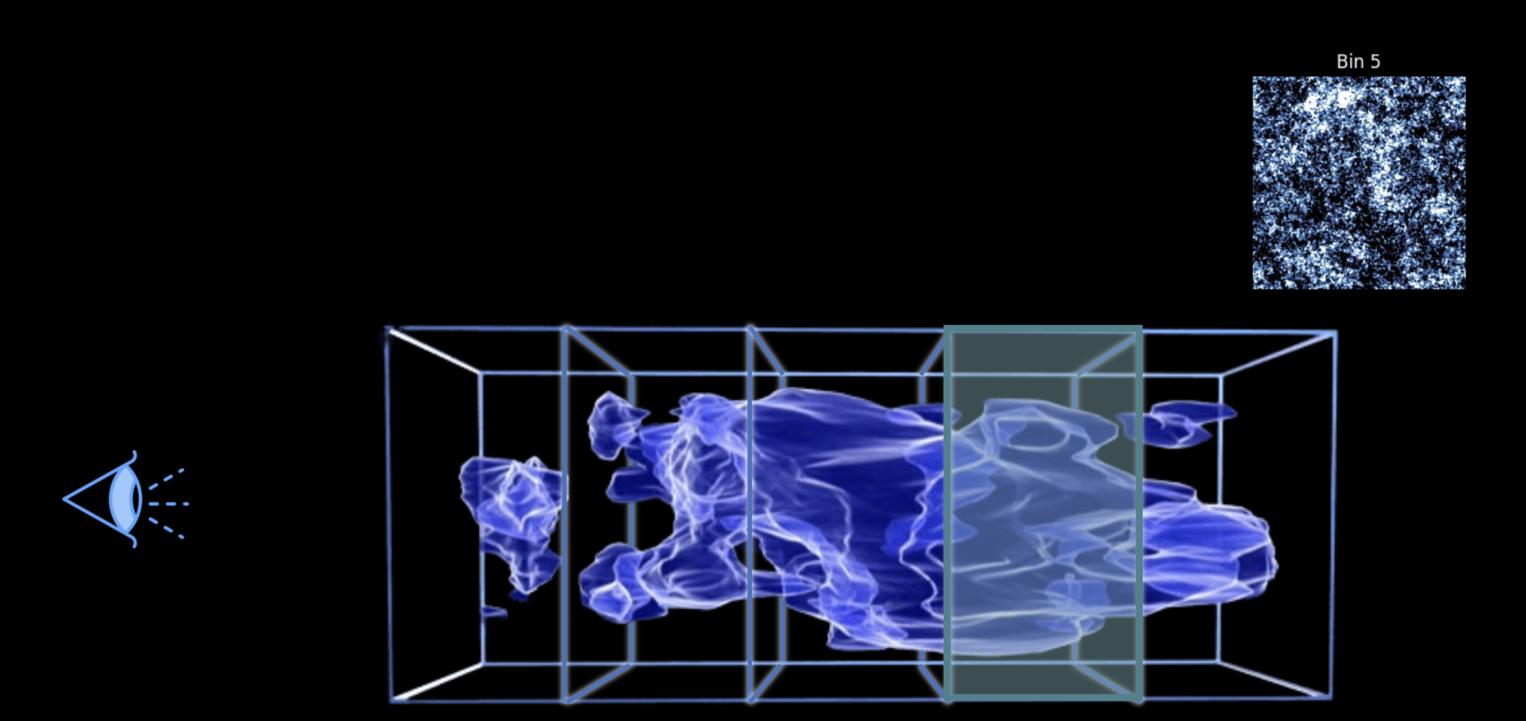
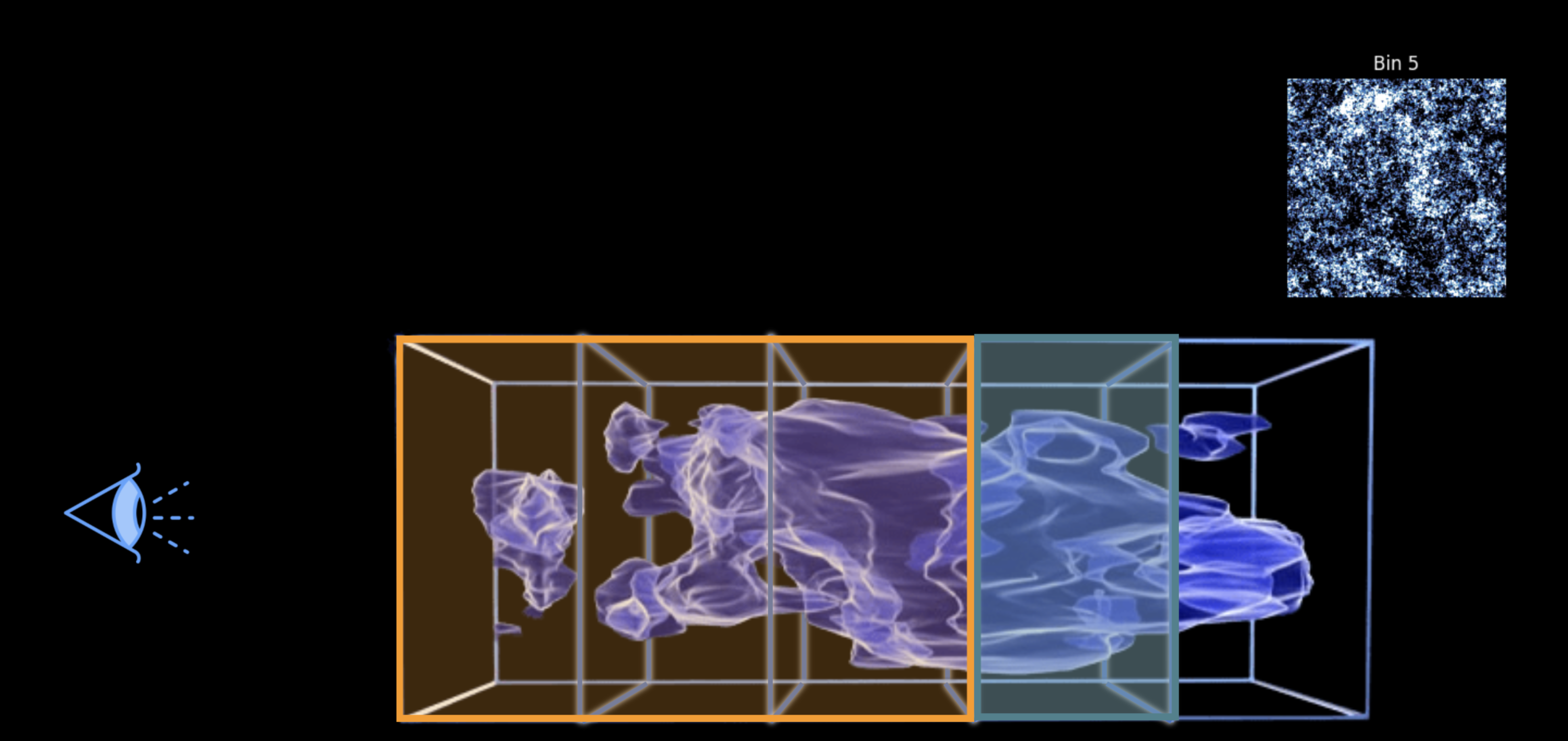
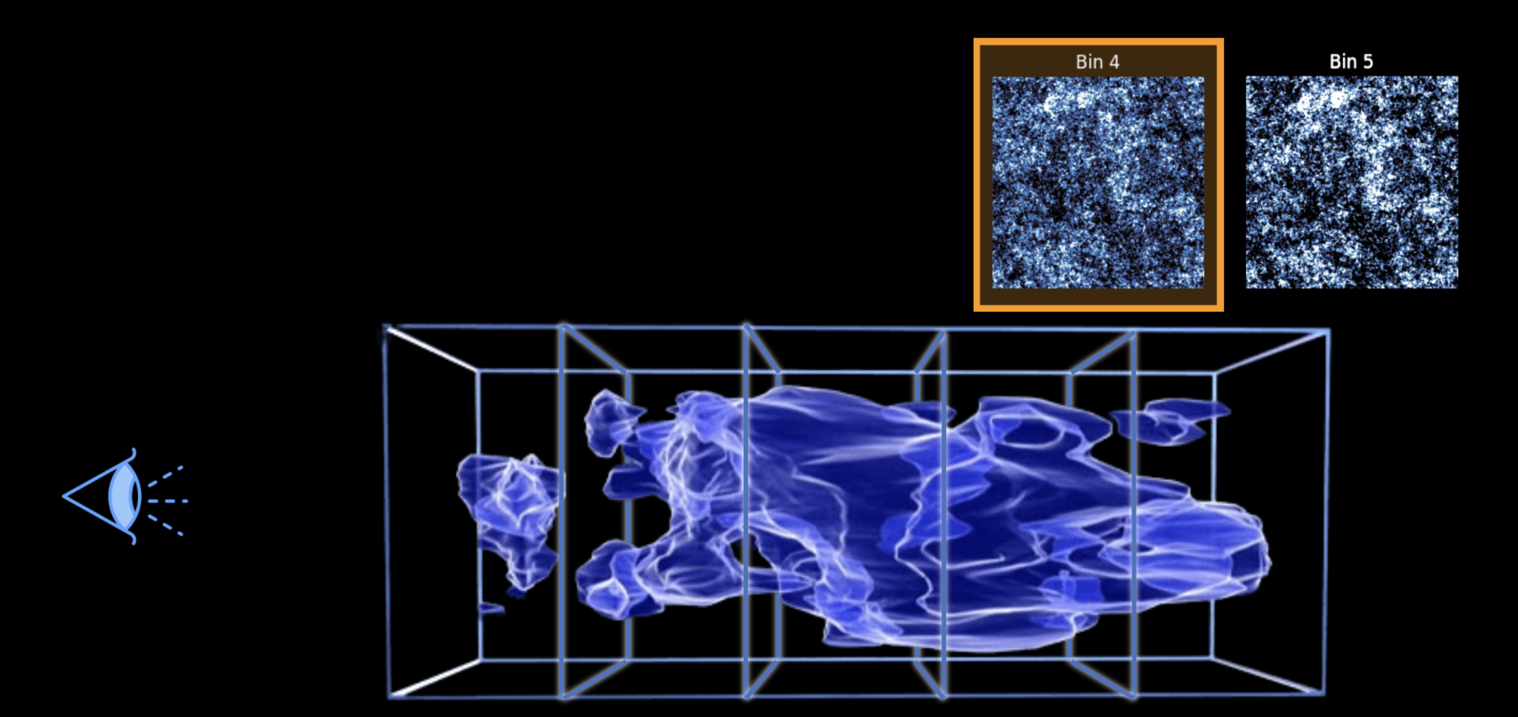
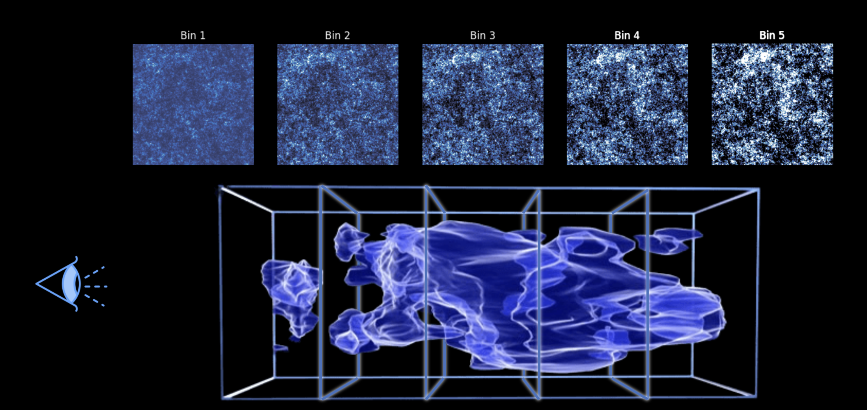
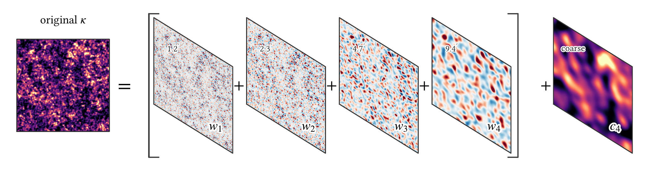
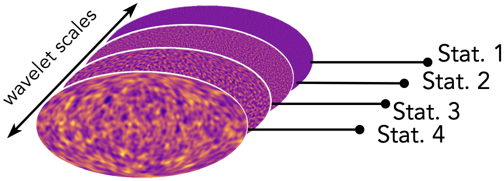
$\mathcal{S}_{j,i}$ — the coefficients of scale $j$ whose SNR falls in bin $i$

sum of absolute coefficients per band and SNR bin → encodes information from every pixel (peaks, voids, ...)

SAY: both of our higher-order statistics are ONE-POINT statistics - histograms of pixel values - and both are made multi-scale by the same starlet transform, which writes the map as a sum of band-pass images, each carrying structure of a characteristic angular size (adjacent bands overlap - they are band-passes, not a partition). That matters twice: each band covers a different frequency range so the covariance is nearly diagonal, and a systematic confined to small scales lands in ONE band, which is what makes the cheap scale cut possible later. Peaks: count local maxima of the SNR field per SNR bin - simple and well established, but it keeps only the discrete features. The l1-norm generalises it: sum the absolute coefficients in each SNR bin instead of counting maxima, so every pixel contributes, voids as well as peaks, and there is no feature-detection step to define or tune. That is our analytical hero for the rest of the talk. CAREFUL: the figure labels its bands 1.2-9.4 arcmin (thesis illustration at a finer pixel scale); OUR analysis uses the four finest dyadic bands, roughly 10 to 80 arcmin, and drops j=1. Do not quote the figure's numbers out loud.

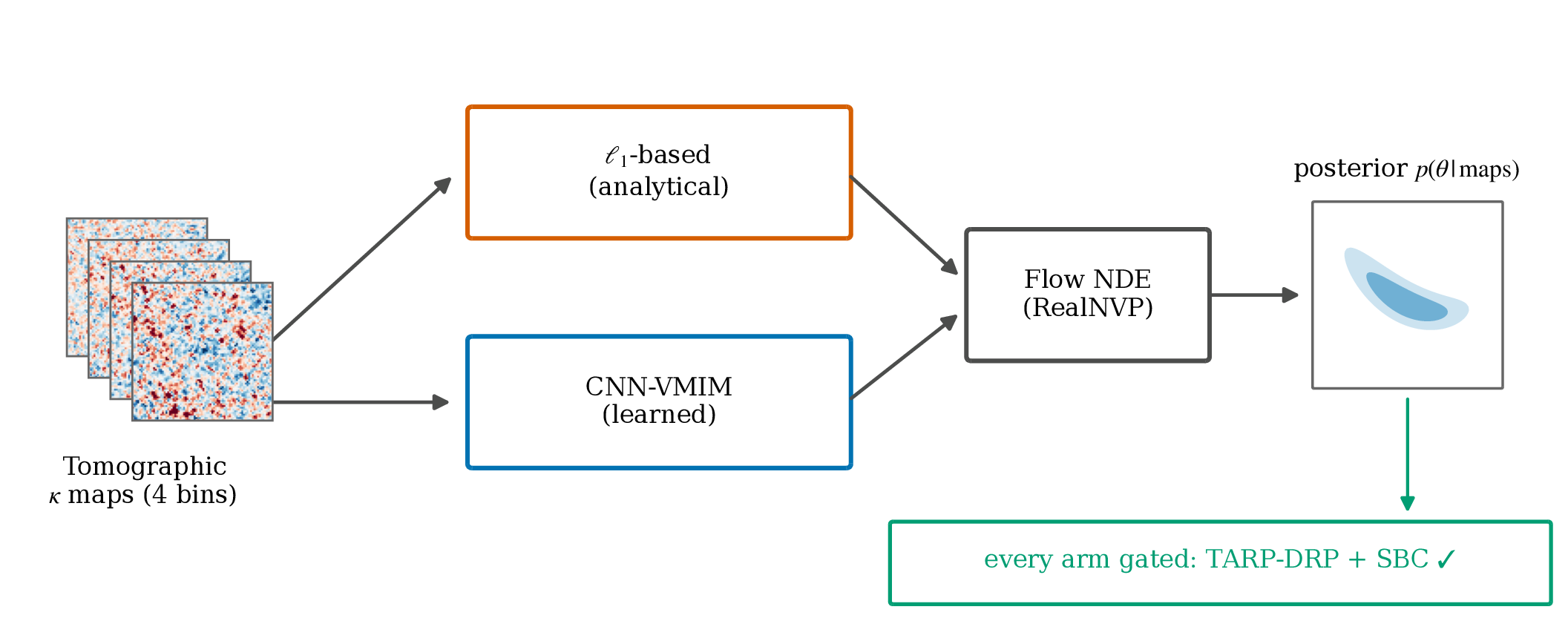
The inference pipeline: neural posterior estimation

wavelet-scale maps and summary statistics

+ noise
wavelet transform

condition

Gaussian$\mathcal{N}(0,\mathbf{1})$

Density estimatorconditional MAF

Posterior$p(\theta\mid x)$

training objective

$\mathcal{L}=-\log p_\phi(\theta\mid x)$

§1 Baryonic Bias Scales with Survey Area

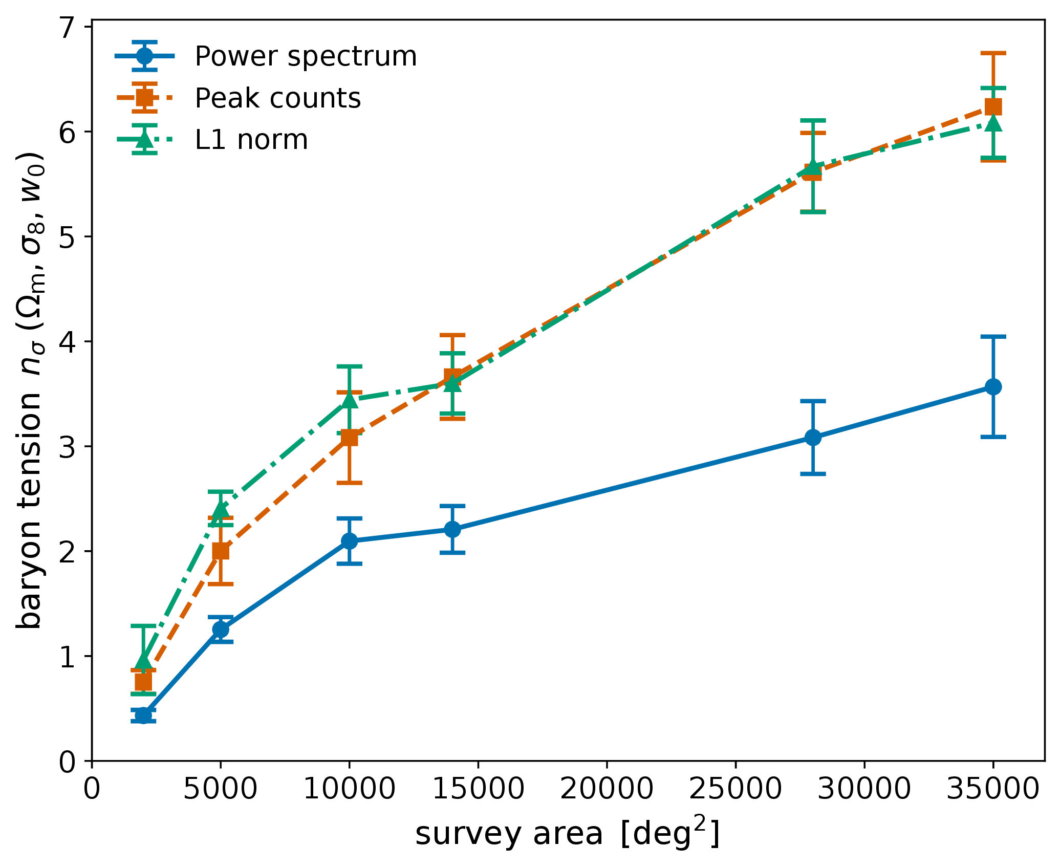
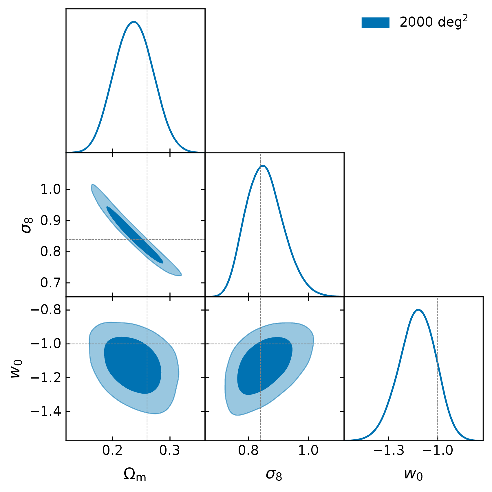
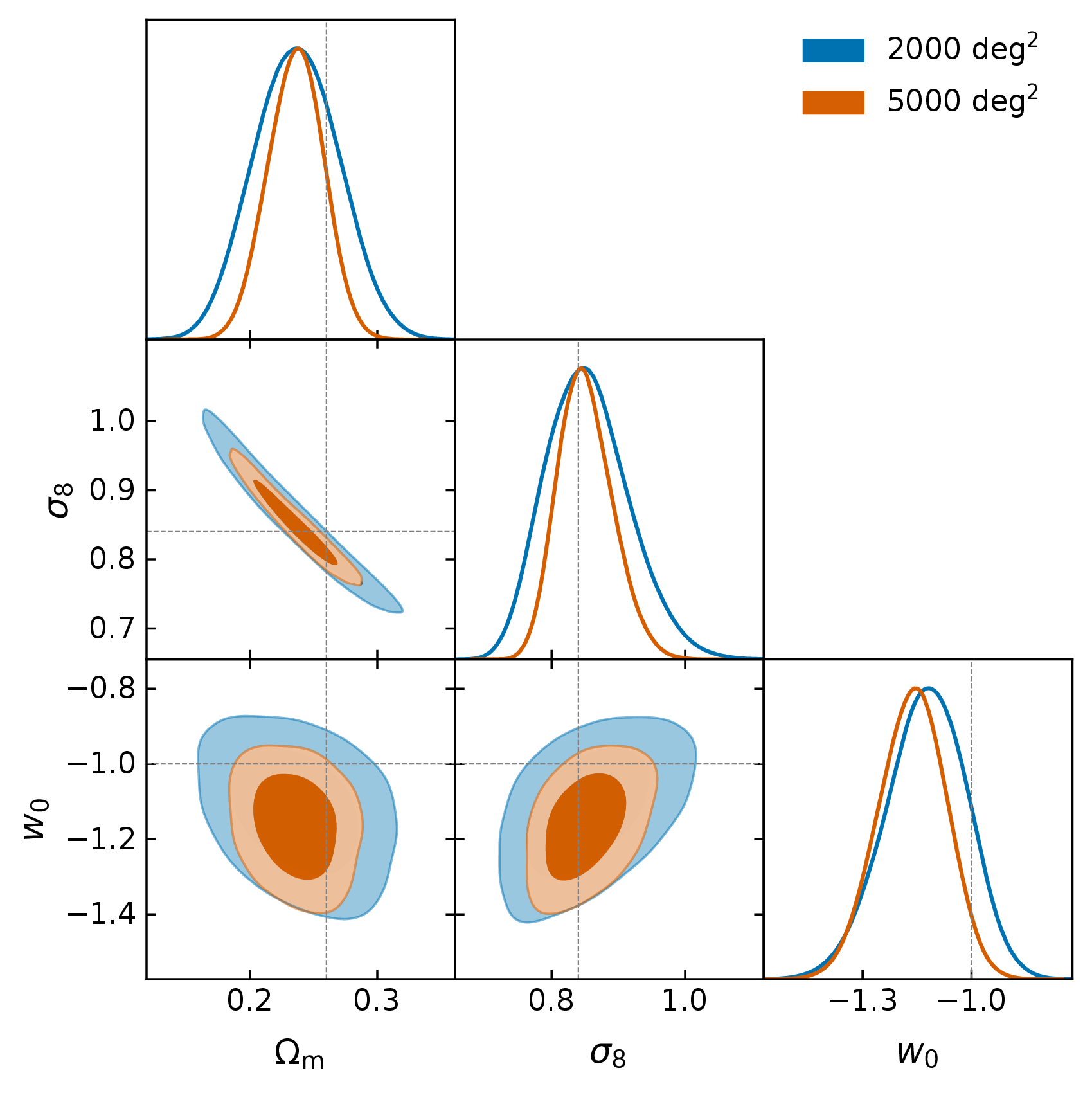
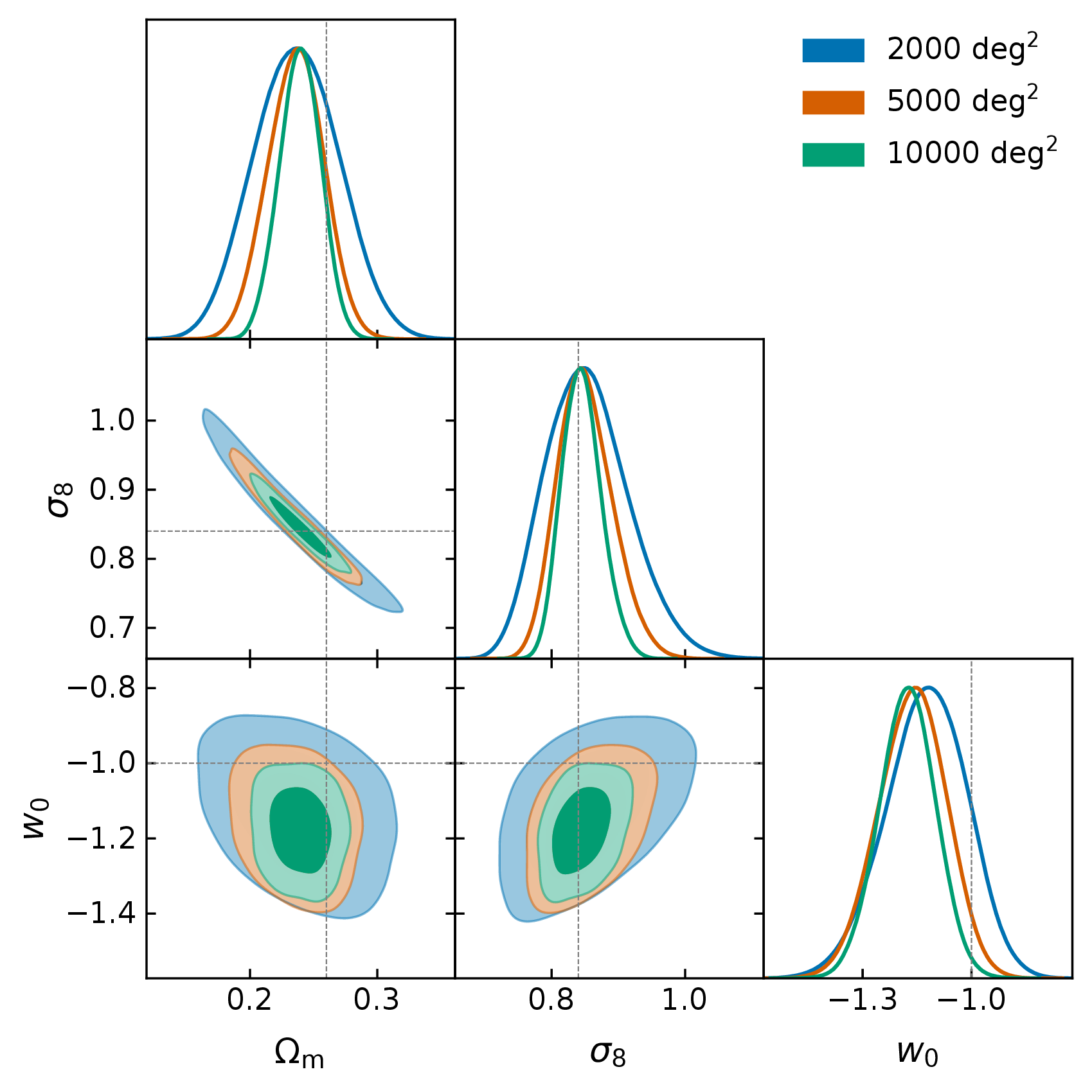
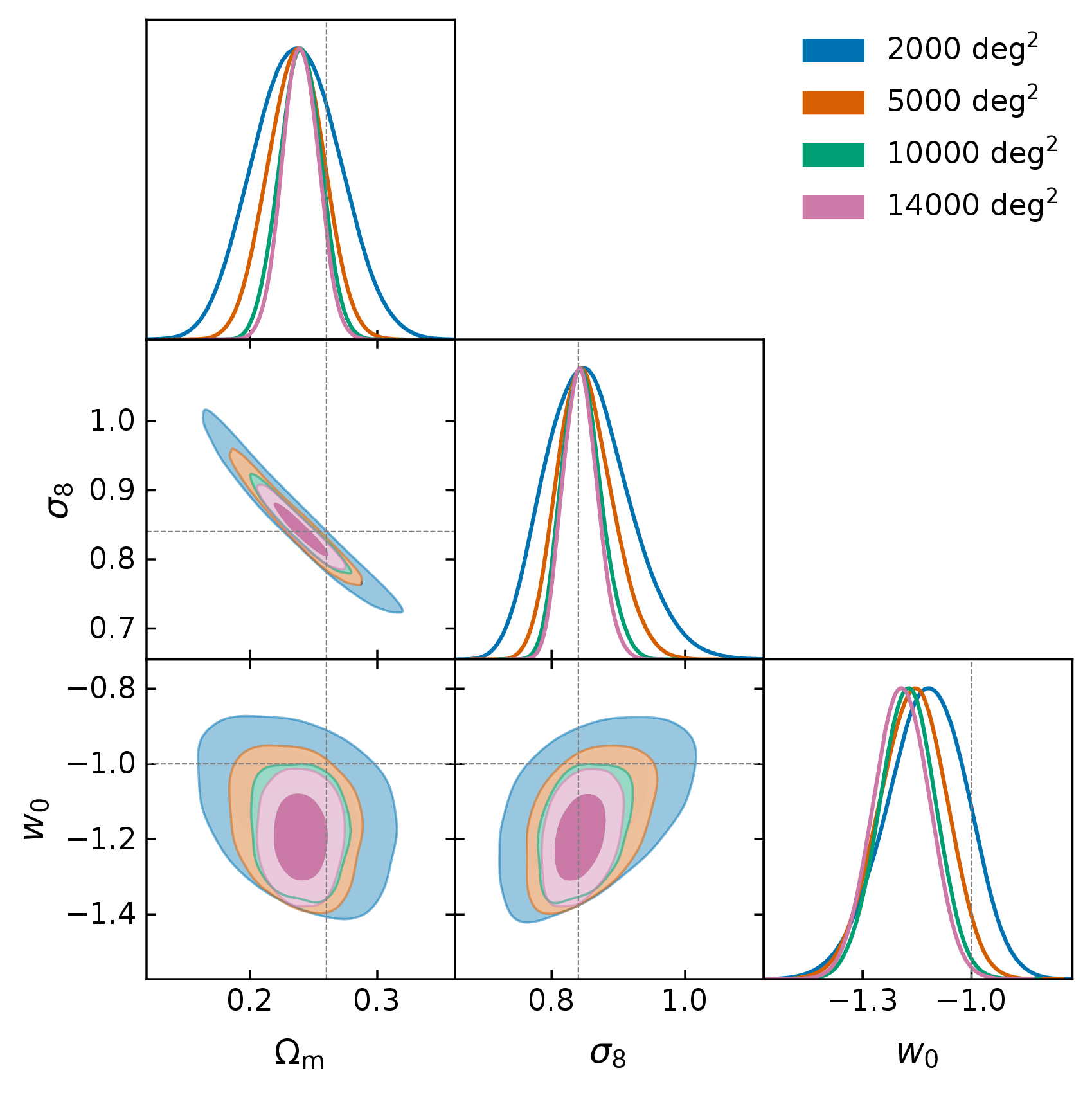
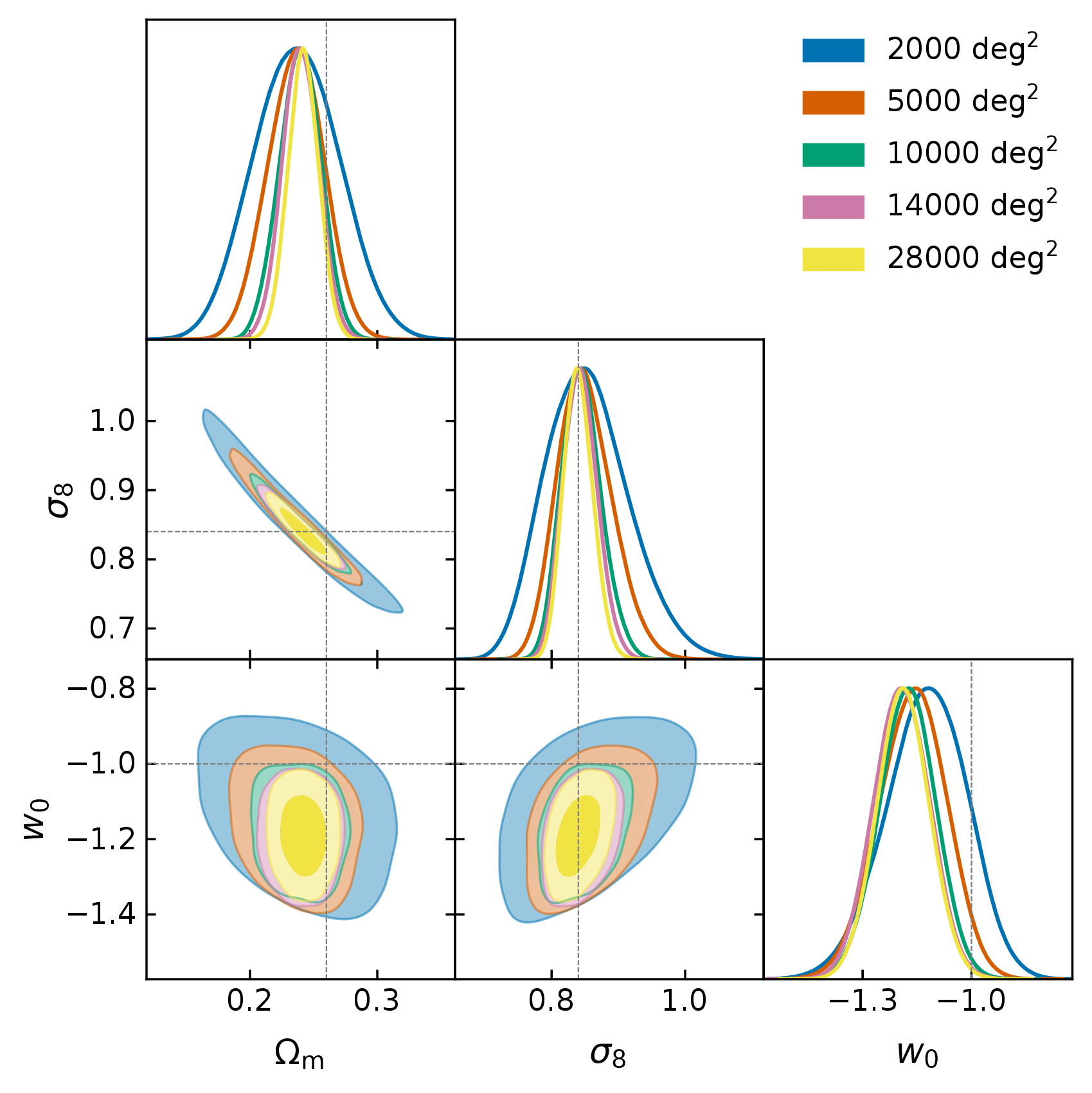
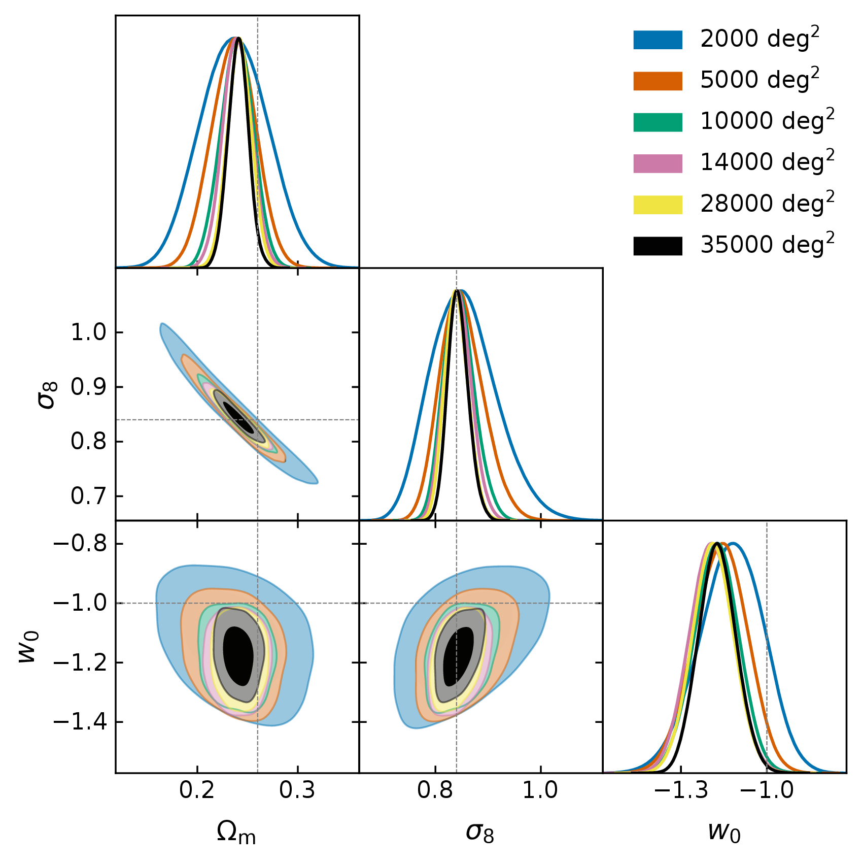
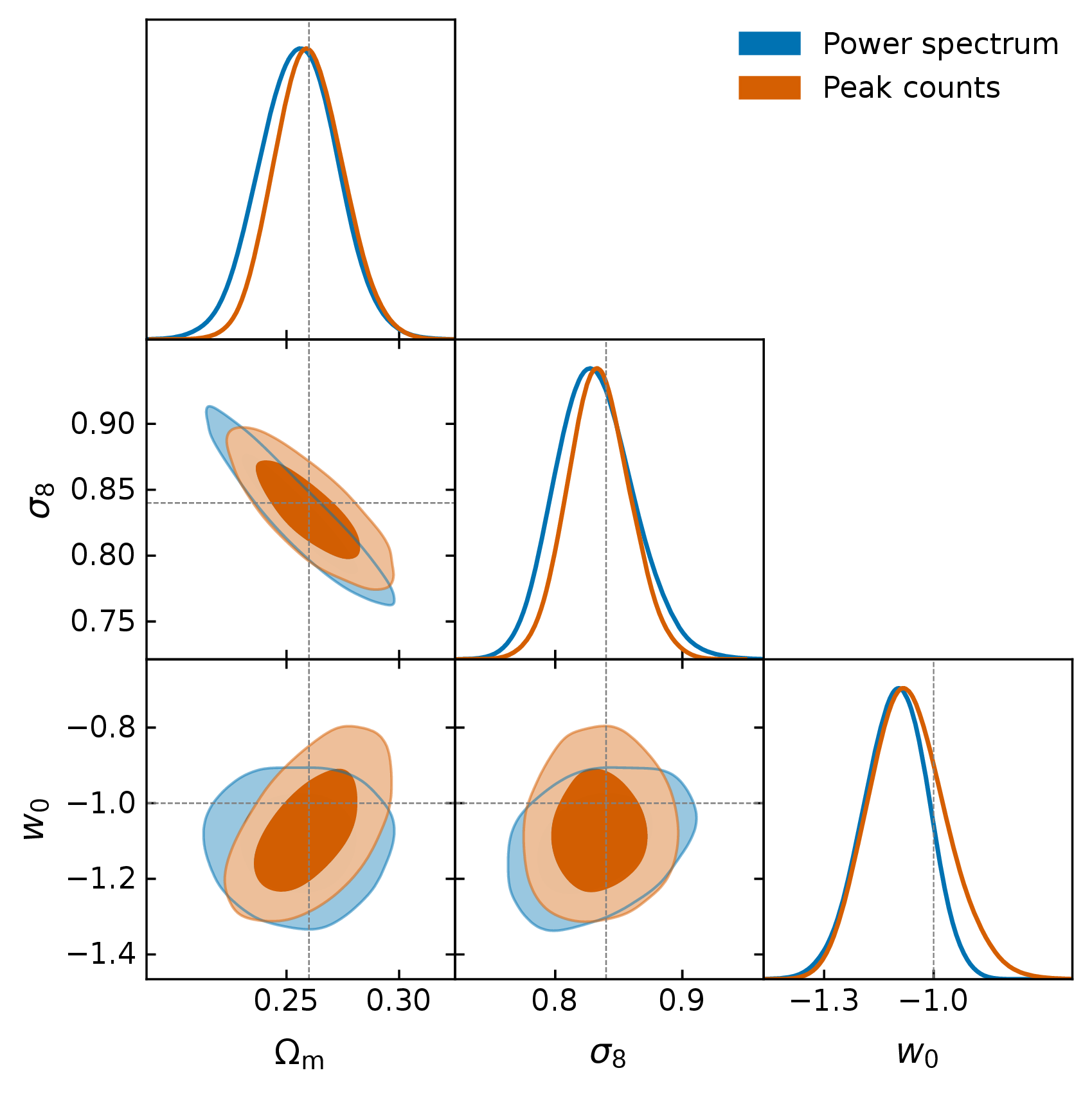
baryon tension in sigma versus survey area for the power spectrum, peak counts and the l1-norm: all three rise with area, the two higher-order statistics well above the power spectrum

At 14,000 deg² (Stage IV): $C_\ell$ shows 2.2σ, peaks and the $\ell_1$-norm 3.6σ
At full sky: $C_\ell$ reaches $\sim3.5\sigma$, both HOS exceed 6σ
HOS show higher bias than $C_\ell$: more sensitive to the baryonically-contaminated small scales

baryon-biased power-spectrum posteriors, tightening and marching away from the truth as the survey area grows from 2,000 to 35,000 square degrees

measured at full map resolution: $\ell_{\rm max}=1024$ for $C_\ell$, all four wavelet bands for the HOS

Tersenov+ 2026, A&A

§1 Buying back an unbiased inference costs $C_\ell$ most of its multipole range, and the starlet its finest band

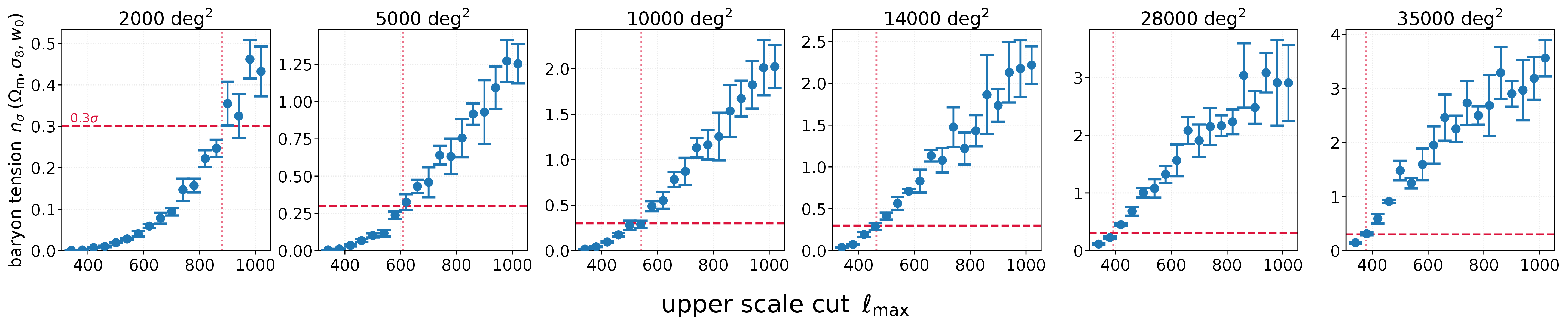
Criterion: bring the baryonic bias below 0.3$\sigma$
$C_\ell$ takes a sliding cut, tuned to what is safe at each area: $\ell_{\rm max} = 860$ at 2,000 deg² falling to 340 at full sky
The starlet concentrates the contamination in its finest band, so dropping $j=1$ suffices at every area

power-spectrum baryon tension versus the upper scale cut, one panel per survey area, with the chosen cut marked against the 0.3 sigma threshold

$C_\ell$→a cut tuned to each area

starlet→whole bands only, so we cut more than we need

Criterion: baryonic bias below 0.3 sigma. Be careful to be fair here. The power spectrum gets a SLIDING lmax - it can be tuned to keep exactly the multipoles that are safe at each area, from 860 at 2,000 down to 340 at full sky, which is a large fraction of the range removed but it is removed precisely. The starlet gets a different kind of cut: the contamination concentrates in the finest band, so dropping j=1 is enough at every area - but because the bands are dyadic, whole-band removal is the ONLY cut available. That is a blunt instrument: at the smaller footprints it certainly throws away uncontaminated quasi-linear information that a finer filter bank would have kept. So the wavelet cut is not "better", it is coarser and therefore conservative. A sqrt-2 or non-dyadic filter bank would allow an area-tuned cut and recover more. One genuine advantage the HOS do have: they are binned in signal-to-noise as well as scale, and the baryonic response sits in the positive tail, so in principle the contamination can be removed where it sits rather than by removing a whole band. We leave that to future work.

§1 Are HOS still useful?

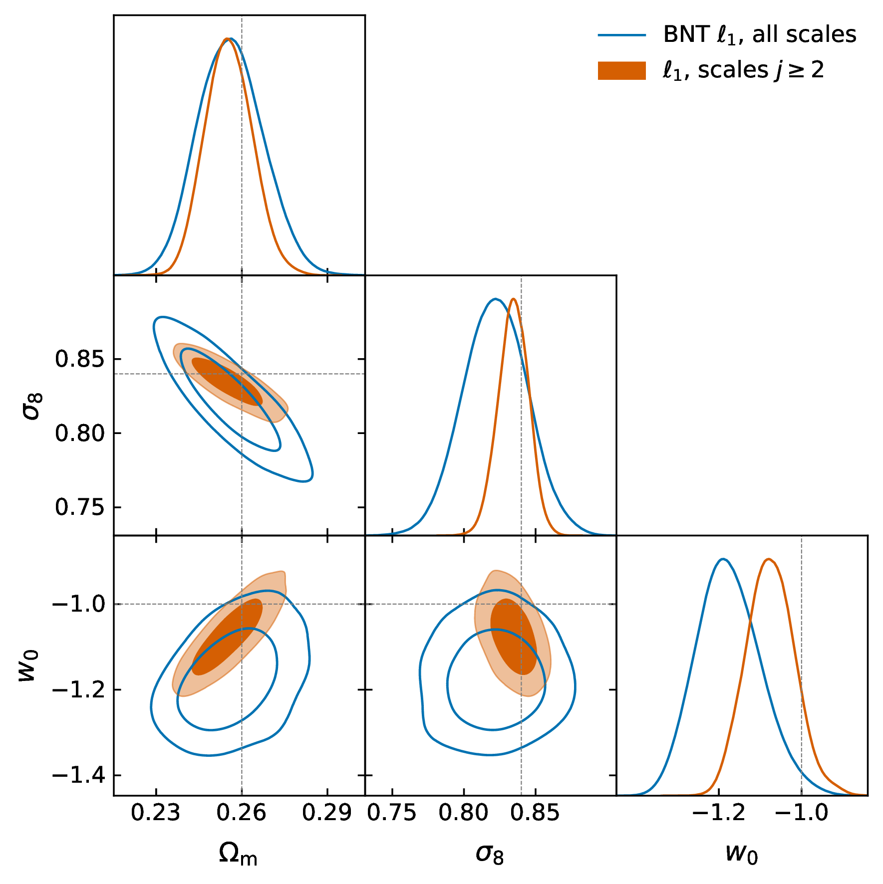
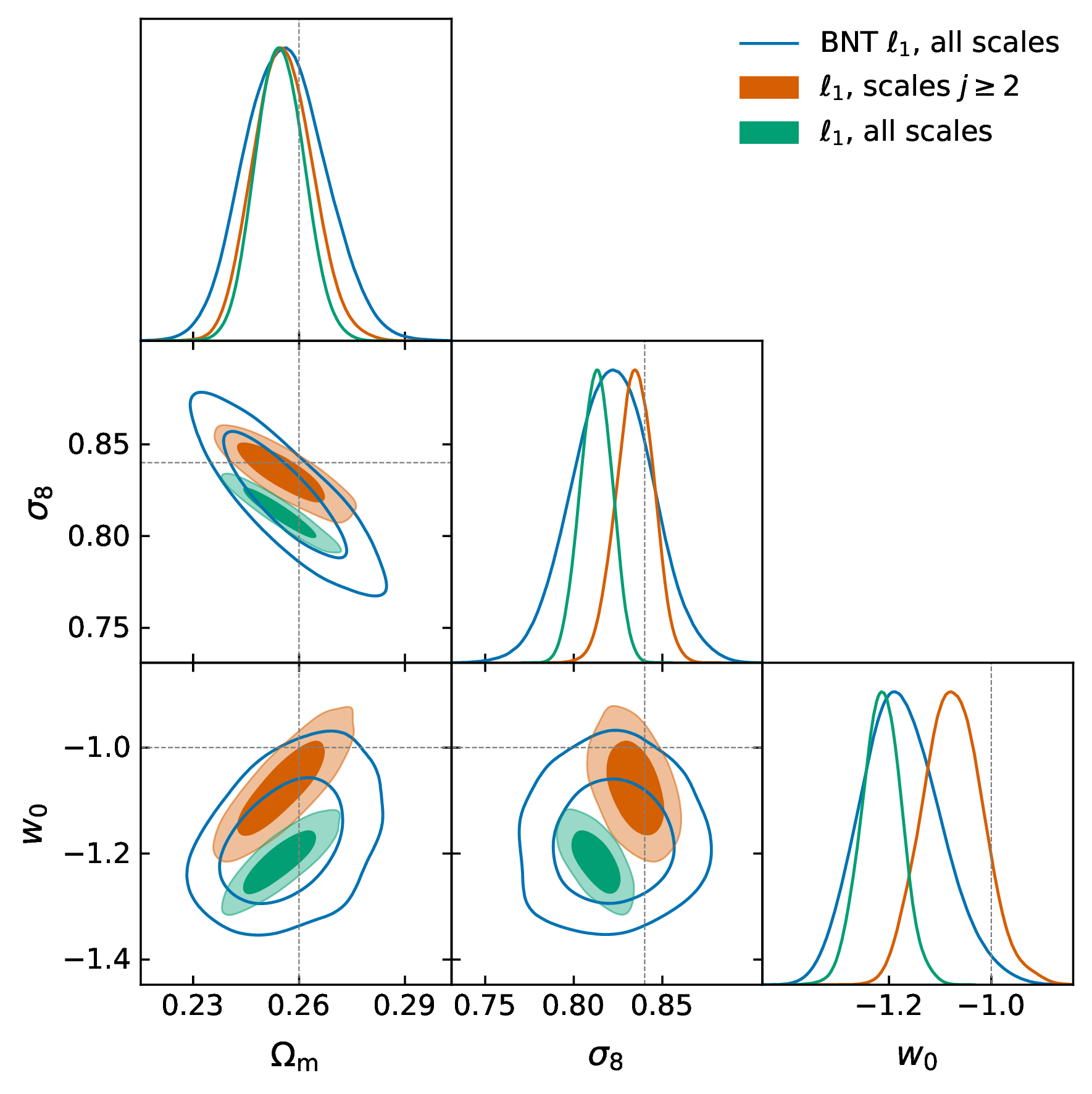
posteriors on baryon-safe scales at 14,000 square degrees: the power spectrum first, then peaks, then the l1-norm, all consistent with the truth

On baryon-safe scales

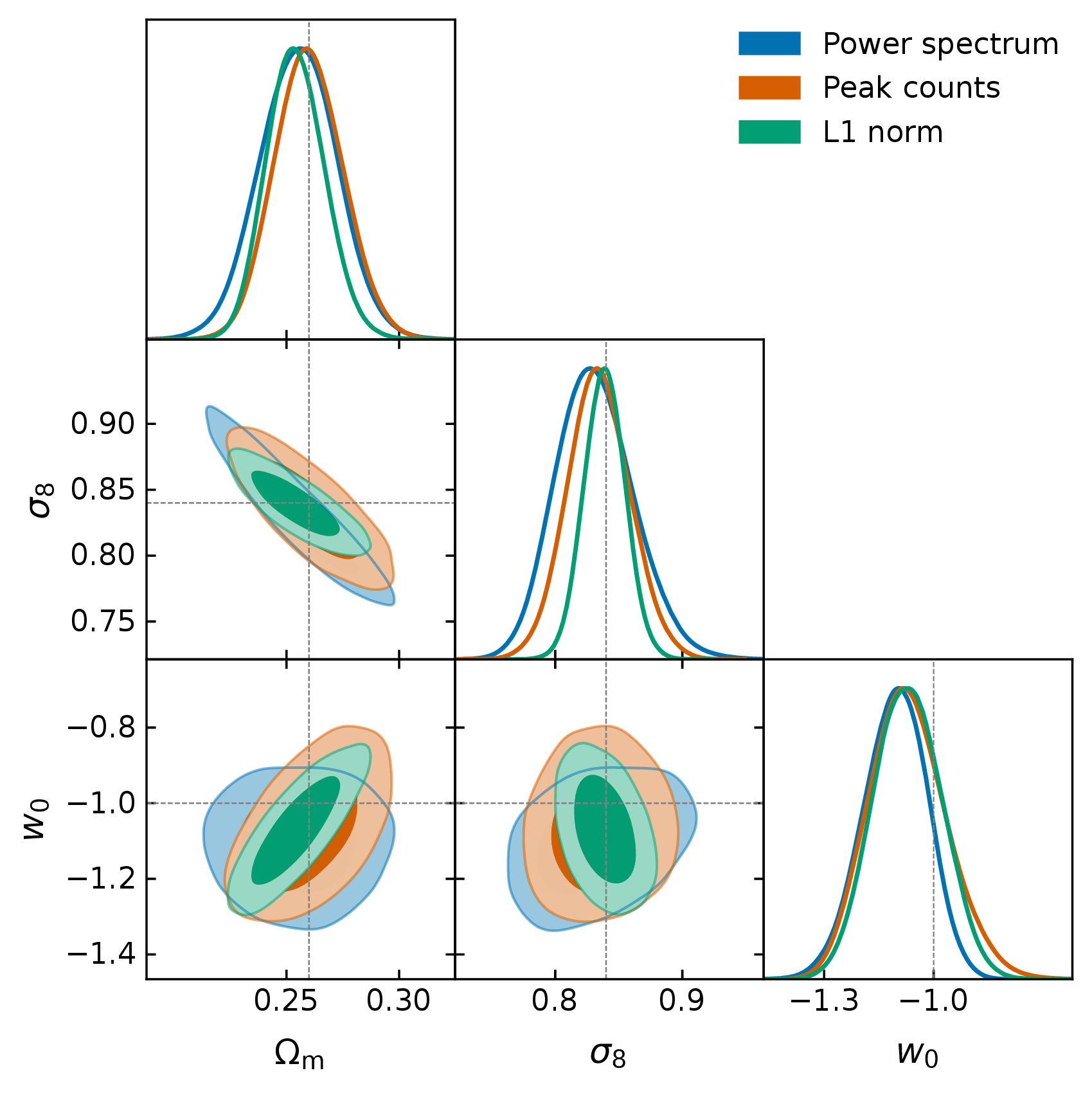
Starlet $\ell_1$-norm: ×1.8 tighter than $C_\ell$ at Stage IV, ×2.6 at full sky
Different degeneracy directions in the $w_0$ planes → HOS always complementary to $C_\ell$

Takeaway

HOS are not merely deep-non-linear probes: the signal persists on quasi-linear scales
A floor:
- our whole-band cut is not optimised,
- better baryon modelling will push the analysis deeper into the non-linear regime, where the HOS gain is larger

On baryon-safe scales the starlet l1-norm constrains x1.80 tighter than C_l at Stage IV and x2.61 at full sky. Be precise about the peak counts: they reach approximate parity with the power spectrum at Stage IV-like areas (x1.07) and slightly exceed it at full sky (x1.17); at the smaller footprints they trail it. Do NOT say they "lose". The reason they trail is largely the cut, not the statistic: the quantised whole-band removal takes out a larger fraction of the peak-count information than the sliding lmax takes from the power spectrum, and that penalty is worst exactly where the power-spectrum cut is loosest. And even at comparable figure of merit they are not redundant - in the planes involving w0 their degeneracy directions differ from the power spectrum, so they add information a joint analysis would use. Takeaway: baryons are a dominant systematic; HOS are robust on quasi-linear scales, not just deep non-linear probes; and everything here is a floor that a finer filter bank or an SNR-space cut would raise.

Beating the power spectrum is a low bar — how much is actually there to get?

→

summary

→

cosmology

No analytic answer for a non-Gaussian field. But a compressor trained to maximise information gives us a ceiling ... but also a fair question: if a learned summary is already optimal, why hand-build a statistic at all?

Act 2 opener. This question is GENERATED by the answer to act 1 - do not ask it earlier. SAY: so non-Gaussian information does survive the baryon cut, and the l1-norm reads it well. But that raises the obvious objection, and it is the one I would raise: the summary is the unknown box in the middle of this pipeline, and the field increasingly fills it with a neural network trained to compress the maps - which is often described as optimal. If that is true, why would anyone hand-build a statistic? Take the objection seriously. The honest answer is that the optimality claim is nearly always demonstrated against the power spectrum, which any non-Gaussian summary already beats, and rarely against a strong hand-crafted higher-order statistic under matched conditions. So the question is open, and that is what we set out to close.

A neural compressor trained to be information-optimal

simulator

$\theta\sim$ prior

→

map $x$

→

network

$f_\phi$

→

summary

$t$

→

flow

$q_\psi(\theta\mid t)$

→

posterior

$p(\theta\mid t)$

\[\max_{\phi,\psi}\; I(t;\theta)\;=\;\max_{\phi,\psi}\;\mathbb{E}\,\log q_\psi\!\big(\theta\mid f_\phi(x)\big)\]

parameter space $\theta$

§2 A fair comparison: same maps, same flow, both calibrated

kappa maps to either l1-norm or CNN-VMIM, into the same flow density estimator, to a calibration-gated posterior

apples to apples

Same κ maps → ℓ1-norm or CNN-VMIM → the same flow NDE → posterior
Flat-sky 10° patches, both arms calibrated
Training set: 324k patches, 899 cosmologies

§2 Read bin by bin, the ℓ1-norm trails the network

matched-pipeline posterior for the auto-only l1-norm, with its figure of merit at 2448 — same maps, same flow, both calibrated — only the summary changes

the CNN posterior added: tighter, with a figure of merit of 3326 against the l1-norm's 2448 — same maps, same flow, both calibrated — only the summary changes

the gap

The learned summary is 36% ahead in FoM₃
But they are not reading the same thing: the $\ell_1$-norm one bin at a time, the network all four maps together
So close that asymmetry, and see how much of the gap goes with it

Tersenov+, in prep.

§2 Two routes to the inter-bin information: build cross maps, or read the pair jointly

route 1 — change the input

the convergence map of tomographic bin 1 — $\kappa_1$

the convergence map of tomographic bin 2 — $\kappa_2$

the pointwise product of the two maps: near-zero almost everywhere, bright where both bins have structure — $\kappa_1\kappa_2$

multiply the two bins pixel by pixel — bright only where both have structure. Six such channels, one per bin pair, each read by the same ℓ1-norm.

route 2 — change the statistic

bin j coefficient the joint plane of wavelet coefficients for a bin pair, with the two one-dimensional histograms along its edges

the per-bin ℓ1-norm
only ever sees the
two axis histograms bin i coefficient

$$L^{ij}_{ab} \;=\!\!\sum_{\boldsymbol{p}\,\in\,\mathrm{cell}(a,b)}\!\! \tfrac{1}{2}\big(|u_i(\boldsymbol{p})| + |u_j(\boldsymbol{p})|\big)$$

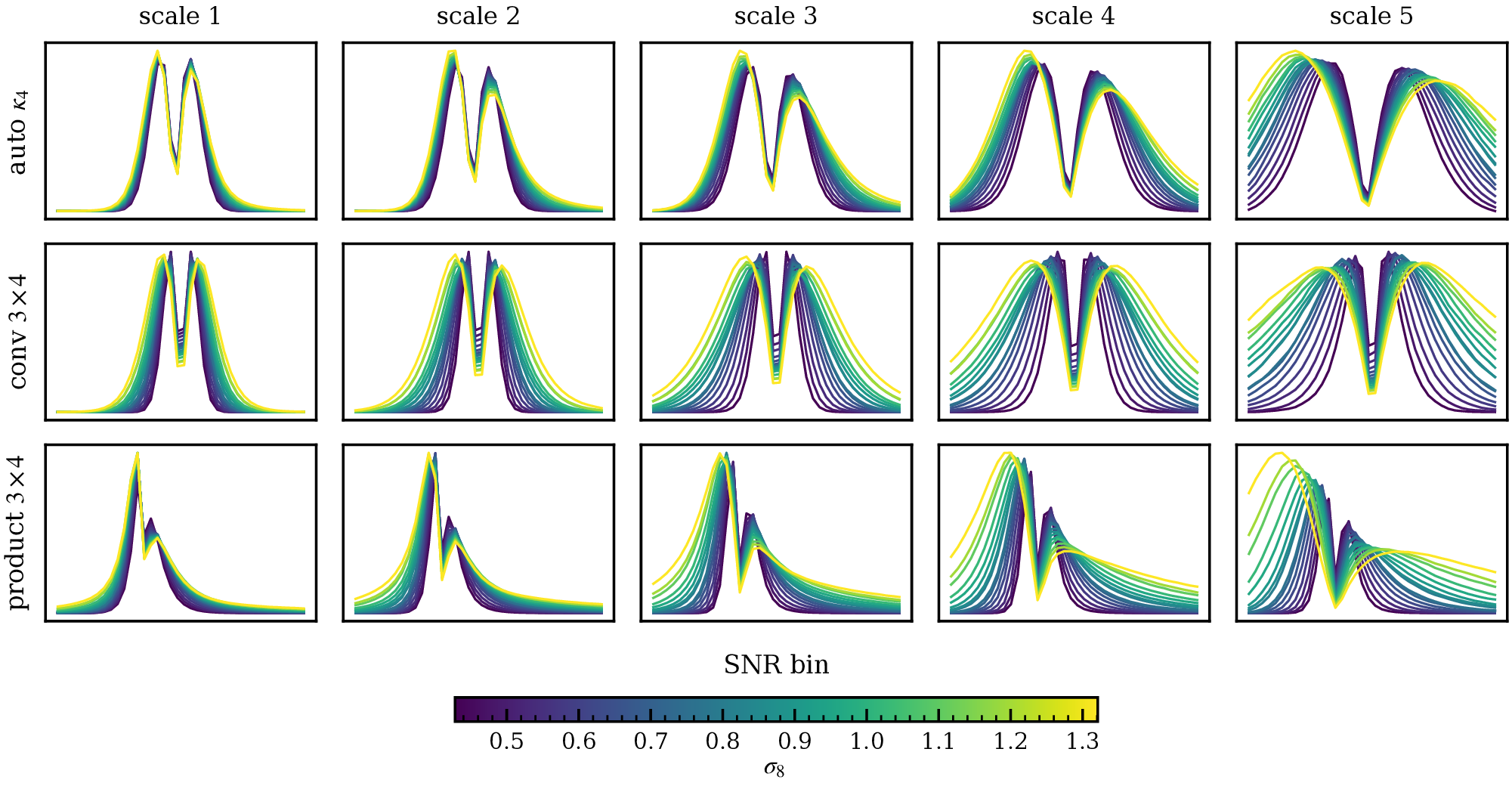
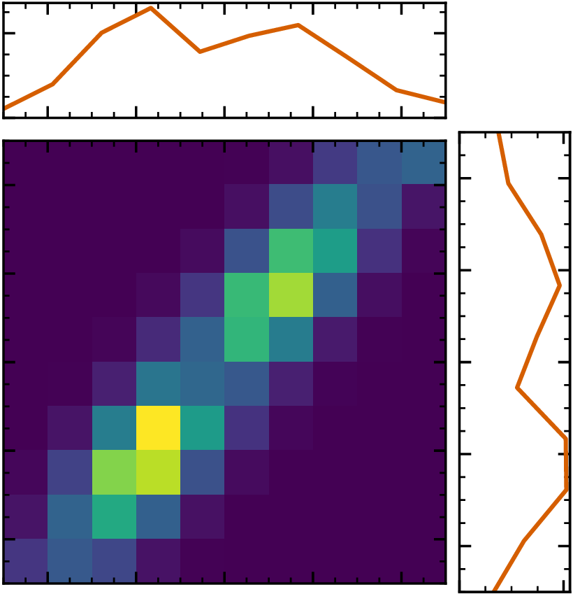
each cell holds the ℓ1 weight of the pixels landing in it

A cross-map collapses each pair into one field before the statistic is taken. The joint ℓ1-norm keeps the whole plane, and needs no new map at all.

SAY: the gap is structural, so there are exactly two places to intervene - the input, or the statistic. ROUTE 1, the obvious one: manufacture the missing channel. For each bin pair, multiply the two maps pixel by pixel; the product is near zero almost everywhere and lights up only where the two bins have coincident structure, so its spatial mean is the zero-lag cross-correlation and its one-point statistics carry the higher joint structure of the pair. Six pairs, six new channels, and the SAME l1-norm runs on each. Built patch-locally, from the patch's own two maps, so a survey observing only that patch could actually form them. IF ASKED: we also test a convolution cross-map, the flat-sky analogue of the harmonic product; it is patch-wide, so its variance sits in a few tens of large-scale modes and it mostly re-supplies two-point information the autos already have. ROUTE 2: leave the four maps alone and change what the statistic reads. At a given scale, every pixel gives the four bins' coefficients at once. The per-bin l1-norm is the |.|-weighted 1-D histogram of each - literally the two curves on the edges of this figure. Lay a fixed 10 by 10 grid on the pair plane instead and sum half of |u_i| plus |u_j| in each cell: that is the joint l1-norm. Ten by ten cells, six bin pairs, four scales, concatenated into the data vector. Summing the absolute value rather than counting pixels is what keeps it an l1-norm rather than a joint PDF estimate. THE POINT, and it is the reason the joint l1 exists: the product map reduces a bin pair to a single derived field BEFORE the statistic is taken; the joint l1-norm never reduces it. CAVEAT if asked: pairwise is the ceiling a patch can populate - a 4-D histogram over K^4 cells against 80x80 pixels is almost everywhere empty, so genuine 3- and 4-bin structure stays with the network. Numbers next slide.

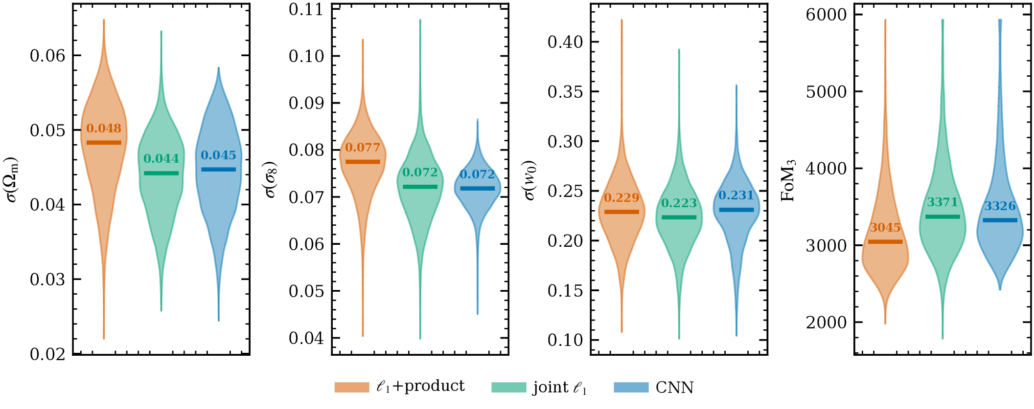
§2 Read the bins jointly and the analytical ℓ1-norm reaches the optimal CNN

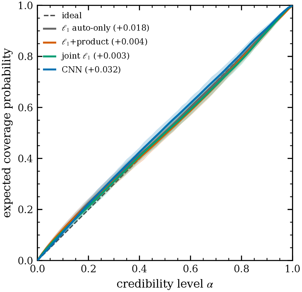
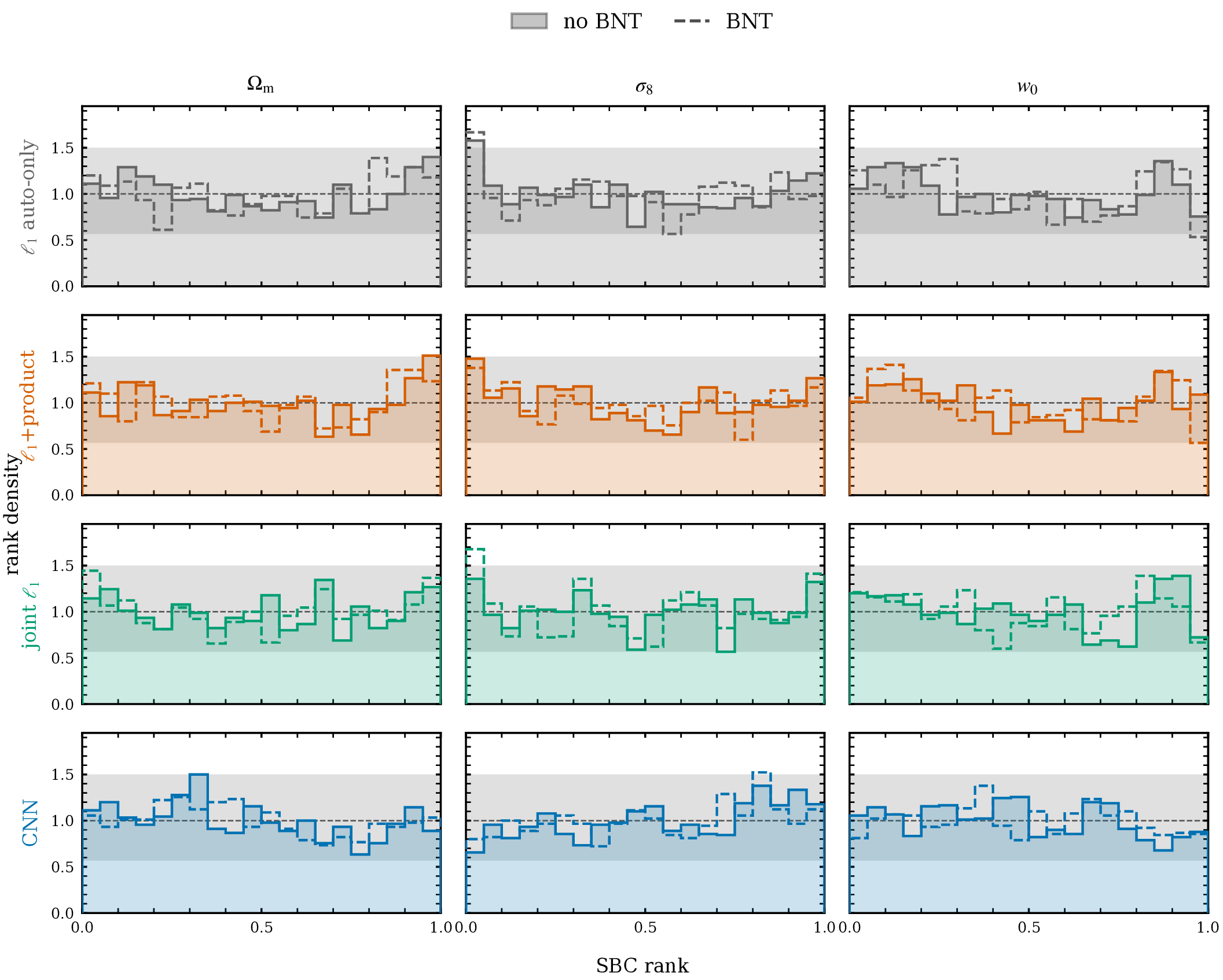
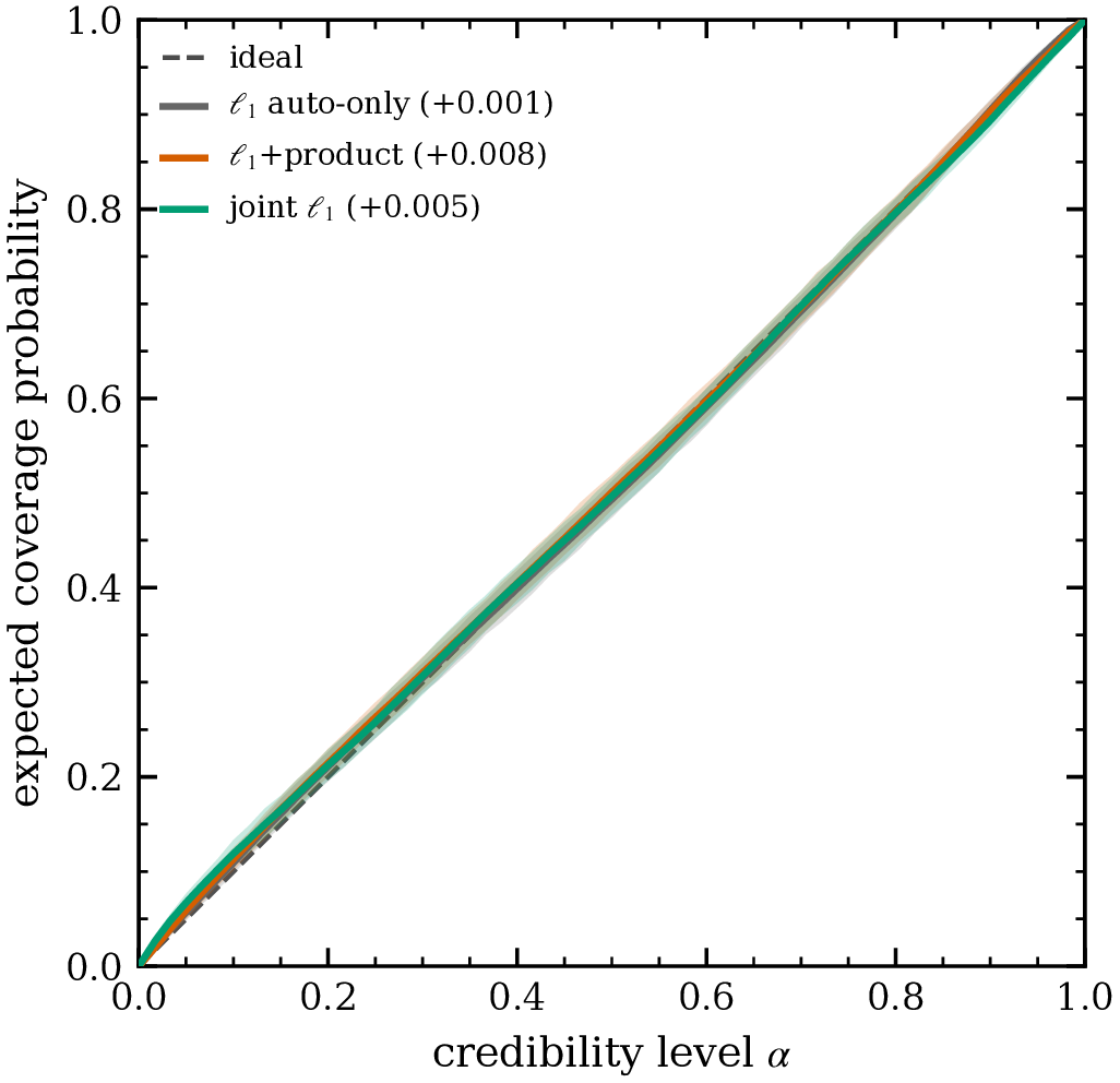
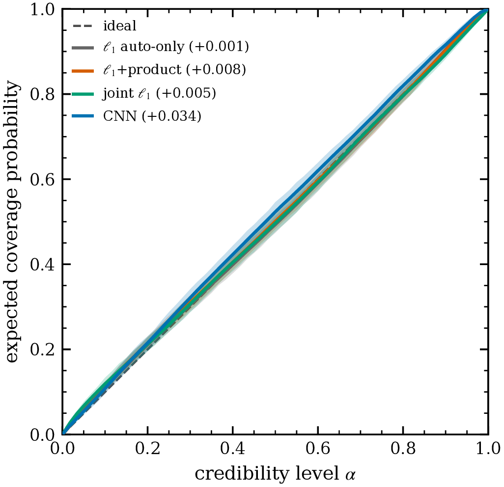
matched-pipeline posteriors: the auto-only l1 first, then plus product cross-maps, then the joint l1, then the CNN landing on top of it; the FoM3 bar inset fills in alongside

The tie holds on every parameter, over 9,000 mock observations.

THE headline. Build it arm by arm: auto-only 2448, plus the product cross-maps 3045, the joint l1 3371, and then the CNN lands at 3326 - on top of the joint l1, not above it. Say precisely what that means and what it does not: a TIE, never a win. The CNN's coverage is mildly conservative, which plausibly accounts for the joint l1 sitting a hair above. And "sufficient as far as we can measure" - both summaries appear to saturate the information the maps make accessible. VMIM trains the network to maximise the mutual information between its summary and the parameters, so it is an estimate of the CEILING, not just another statistic; a hand-built statistic reaching that ceiling is a sufficiency result. Referee aside if pushed: getting the CNN there took an expressive flow (RealNVP, +36%) and a better architecture (resnet18, +6%); the deeper net overfits at 899 cosmologies, so "you trained it wrong" does not hold. The per-mock violins are in backup if anyone wants the population rather than the medians.

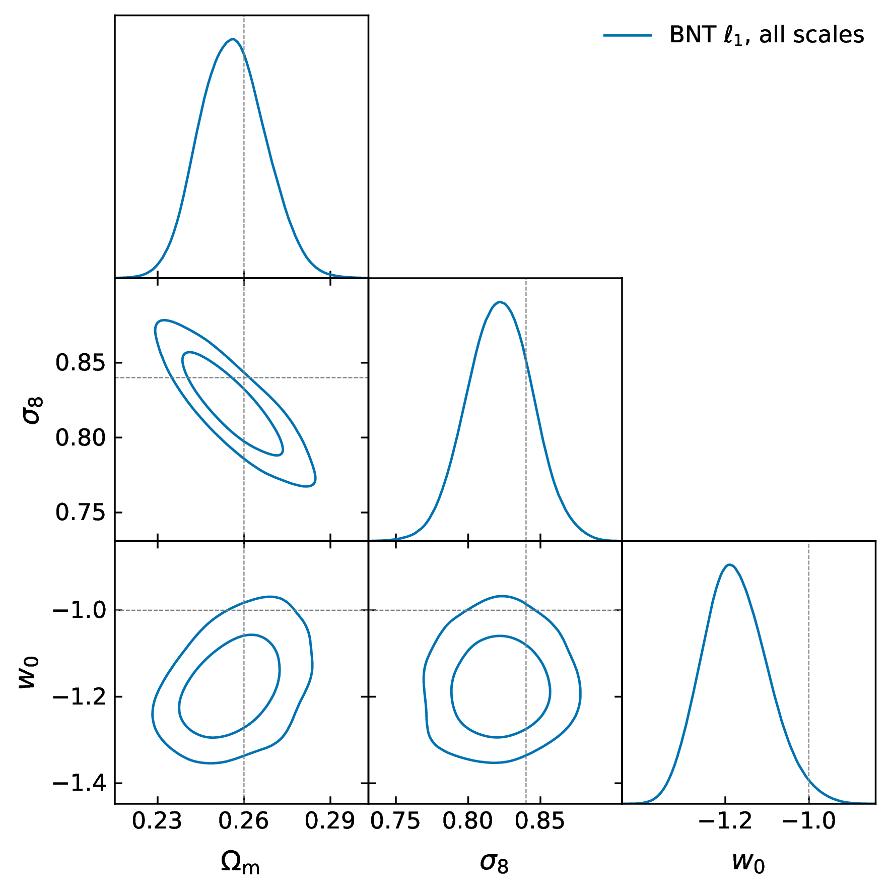
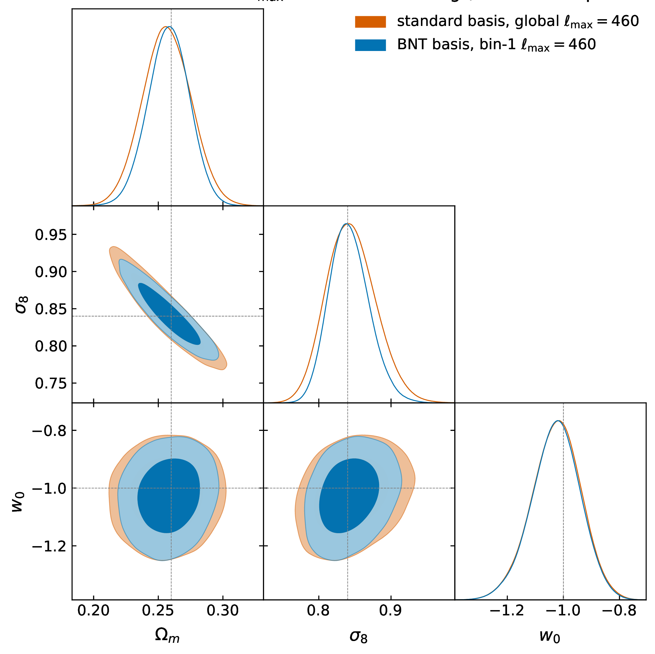
§3 Nulling promises localized scale cuts... For HOS it inflates the contours instead

the promise

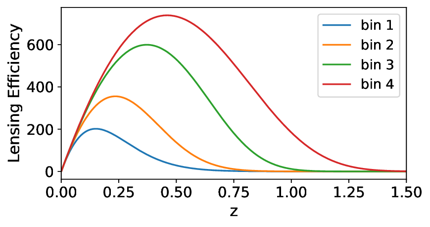
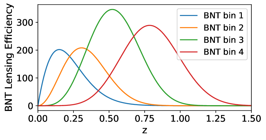
standard lensing efficiency kernels: broad and overlapping across redshift — broad, overlapping

↓

BNT lensing efficiency kernels: nulled and localized in redshift — nulled, localized

A fixed angular scale stops mixing redshifts, so the cut can go only where the systematic is

the problem

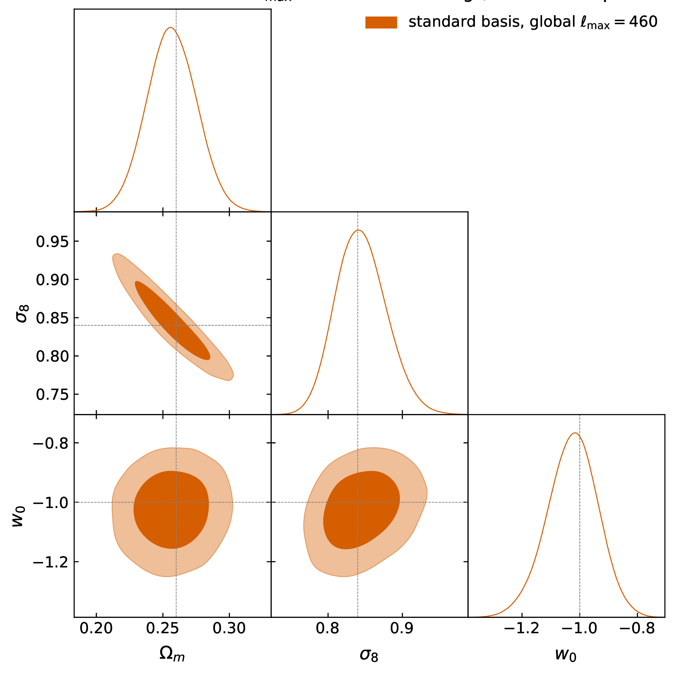
the l1-norm posterior in the BNT basis, visibly inflated against the same statistic in the standard basis — blue = the ℓ1-norm in the nulled basis

BNT = a fixed, invertible transform → nothing can have been lost...

Tersenov+ 2026, A&A and Tersenov+, in prep.

SAY: this is the third thing we looked at, and it stands on its own. Nulling - the BNT transform, Bernardeau, Nishimichi and Taruya 2014 - is a linear re-mixing of the tomographic bins that cancels the low-redshift lensing efficiency. Why anyone wants it: standard lensing kernels are broad and overlapping, so one angular scale mixes low-z small scales with high-z large ones, and an angular cut throws away clean high-z information along with the contamination. Null the bins and each transformed field is localized in redshift, so the baryon sensitivity lands in ONE transformed bin and you cut scales only there. That is a genuinely promising way to do scale cuts. CLICK. Applied to a map-based higher-order statistic it backfires: the same mixing correlates the originally-independent shape noise across bins, the noise floor rises, and the contours inflate - worse than standard tomography even with conservative cuts. PLANT, as a minor technical aside: for the power spectrum it IS lossless, PROVIDED you keep the cross-spectra between transformed bins. Do not explain that yet - it pays off on the next slide. Then the paradox, and PAUSE: this is a fixed invertible matrix, the Jacobian cancels in Bayes, the Fisher information is unchanged, the posterior from the full field is identical in both frames - and yet the l1-norm keeps 16 percent. NAME Vinciguerra et al. 2026 (Euclid): they hit the same wall keeping tomographic maps for bin combinations up to quadruplets, and concluded that recovering the SNR is "highly non-trivial".

§3 The information is recoverable by the summary that reads the bins jointly

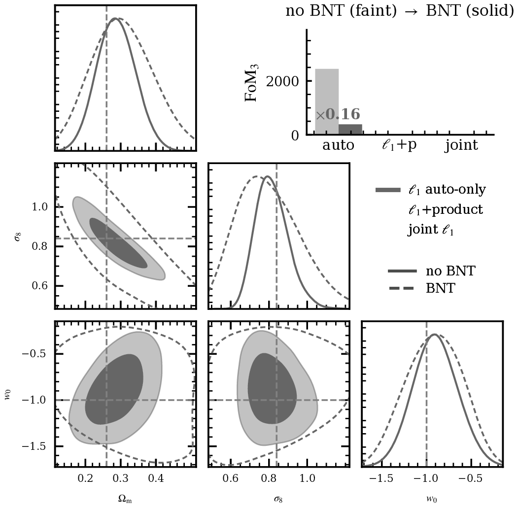
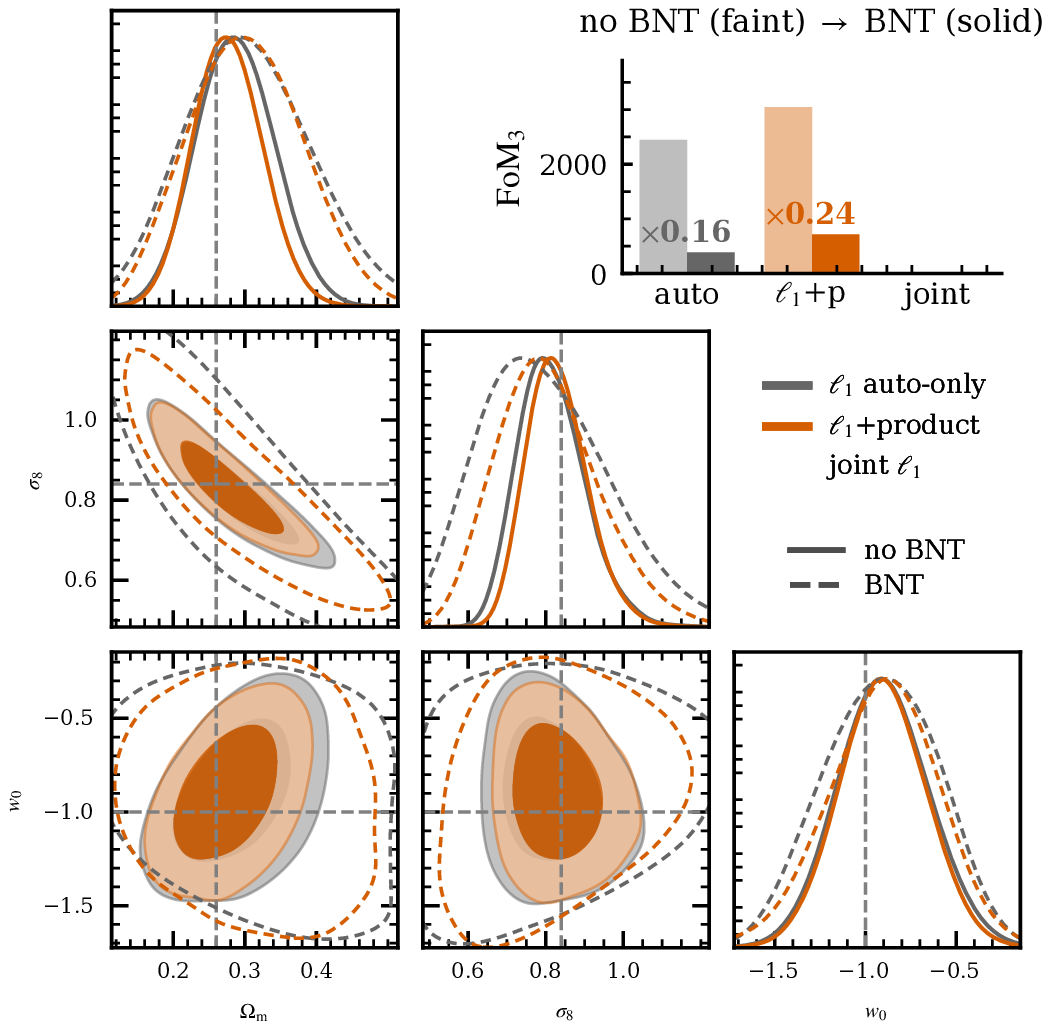
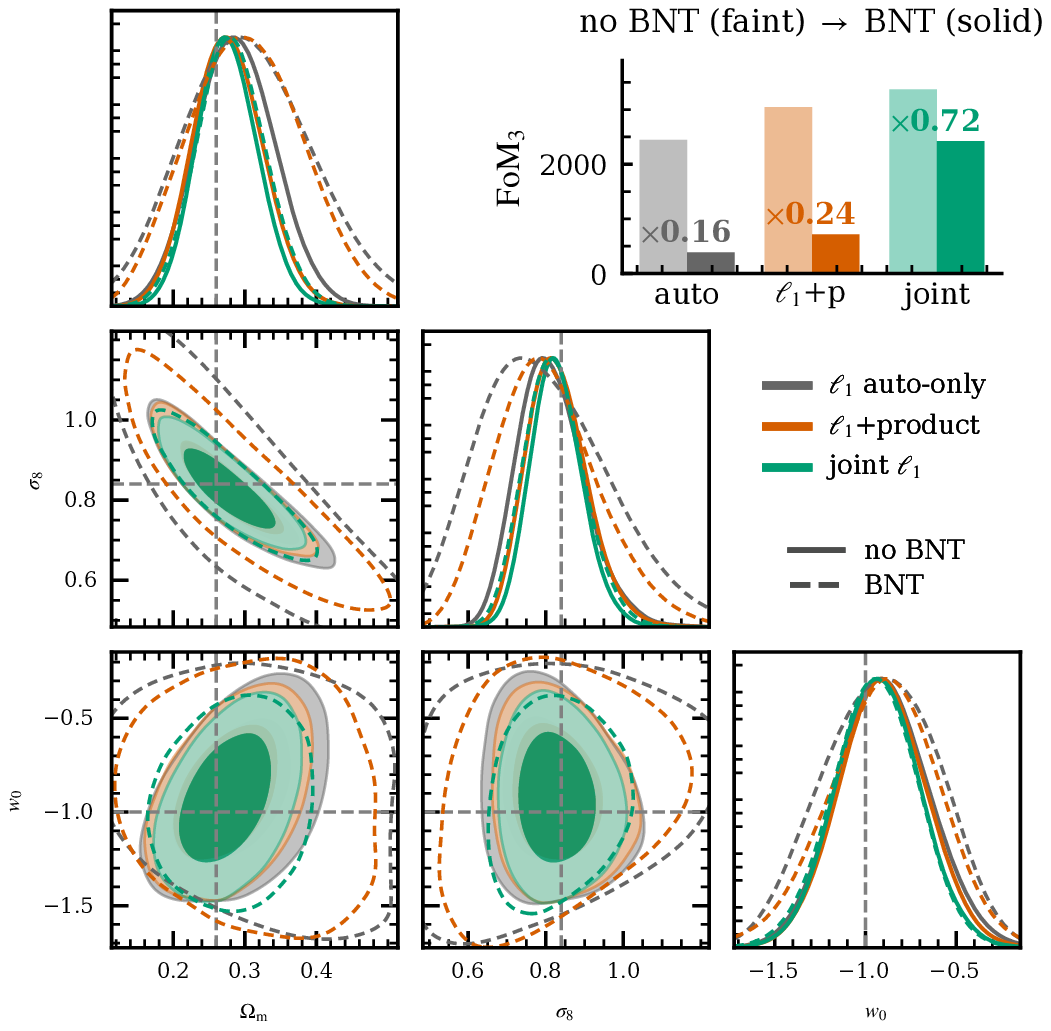
figure of merit retained under the nulling

one bin at a timeℓ1, auto-maps

0.16×

+ one derived field per pairℓ1 + product cross-maps

0.24×

each pair's full 2-D distributionjoint ℓ1-norm

0.72×

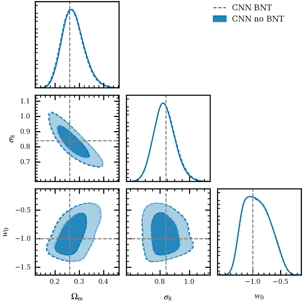
all four channels at onceCNN, VMIM-trained

~1×

Same four summaries as before. In the standard frame they spanned 38%; here, a factor of six.

nulled frame over standard

posteriors in the nulled frame: the auto-only l1 balloons, retaining 0.16 of its figure of merit, then the product and joint arms tighten — dashed = the nulled frame

So nulling can be kept as a mitigation at no cost in constraining power, provided some stage of the pipeline reads the bins jointly. And the power spectrum was this ladder's first rung all along.

SAY: so we asked what it takes to get the information back, and ran the same four summaries through the nulled frame. Per-bin l1 keeps 0.16. Add one derived field per pair - the product cross-maps - and it is 0.24, better but nowhere near. The joint l1-norm, the statistic we built two slides ago, keeps 0.72. The CNN, which reads all four channels natively, is essentially untouched by the transform: the measured value is 0.96 +/- the quoted error, consistent with 1, which is why the slide says approximately 1 rather than a false-precision 0.96. Quote it as "no measurable loss", and give the number only if asked. The practical message, and this is the result that matters for anyone planning a nulled analysis: nulling need not cost a higher-order analysis anything, PROVIDED some stage of the pipeline reads the bins jointly. CASH the clause from the previous slide: the power spectrum survives the transform for exactly this reason - auto PLUS cross spectra are closed under C-hat maps to B C-hat B-transpose and so exactly invariant, while the auto-spectra alone keep only the diagonal and are not. The two-point case was the first rung of this same ladder all along. COUNTER-INTUITION worth saying out loud: the nulling is designed precisely to DE-correlate the bins, and joint reading matters more there, not less. HONEST RESIDUAL: the joint l1 keeps 0.72, not all of it - the remainder is genuine three- and four-bin structure that a pairwise statistic cannot reach, and that is the one place the network keeps an advantage. The CNN corner and the calibration of every BNT posterior are in backup.

Conclusions

Q1 Does baryonic feedback put the non-Gaussian information out of reach? ✓No. Cut every contaminated scale and the ℓ1-norm is still ×1.8 tighter at Stage IV, ×2.6 at full sky.
Q2 Do we need deep learning to extract it? ✓No. Read the bins jointly and a fixed wavelet statistic matches the optimal compressor, with no training.
Q3 Can redshift nulling then be used with higher-order statistics? ✓Yes, provided the summary reads the bins jointly. There is no loss of information, and the inflation is a frame artifact. What is left: the genuinely three- and four-bin structure a pairwise statistic cannot reach.

Mitigating baryonic effects in weak lensing with higher-order statistics
Tersenov, Guerrini, Starck & Kilbinger — A&A, in press
The joint wavelet ℓ1-norm matches neural compression for tomographic weak-lensing inference
Tersenov, Starck & Kilbinger — in preparation both on arXiv in September

for questions

Backup

Calibration, the completeness ladder, the nulled-frame companions, and the maps.

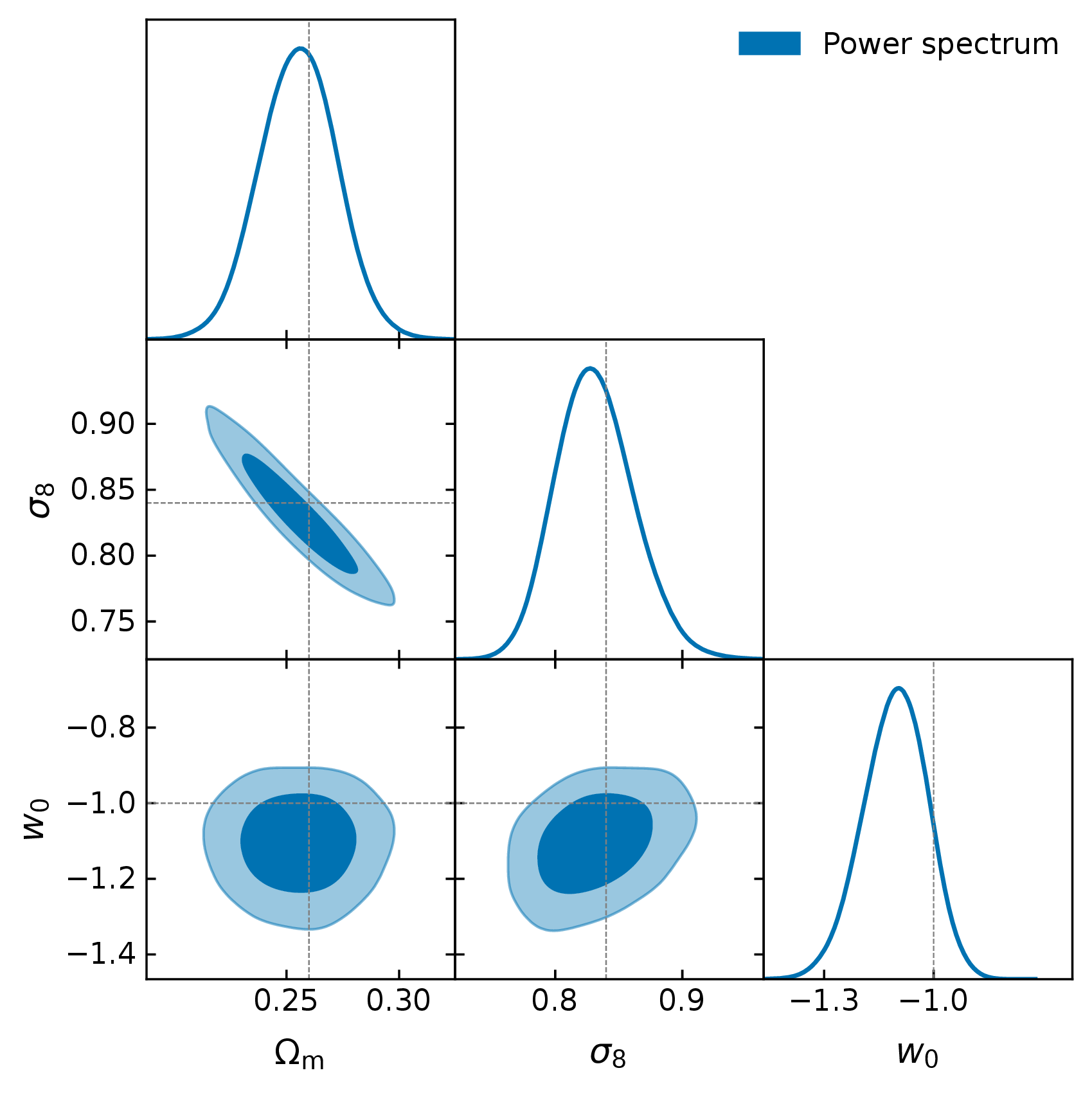
Q1 With no feedback model at all, cutting every contaminated scale still leaves the ℓ1-norm ahead of the power spectrum

figure of merit relative to the power spectrum, on each statistic's own baryon-safe scales

A floor: no feedback model, every contaminated scale discarded.

Q2 Build joint reading in, and a fixed wavelet statistic reaches the ceiling

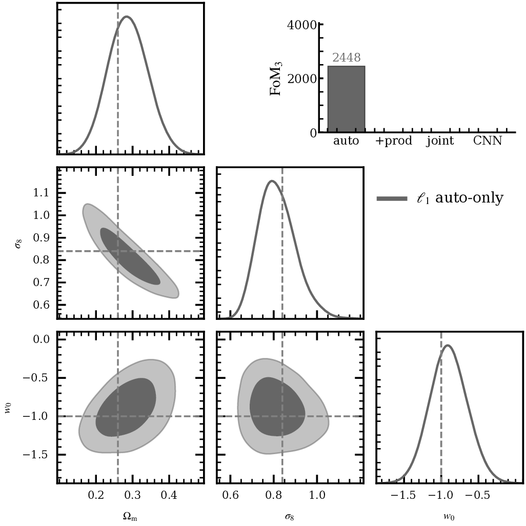
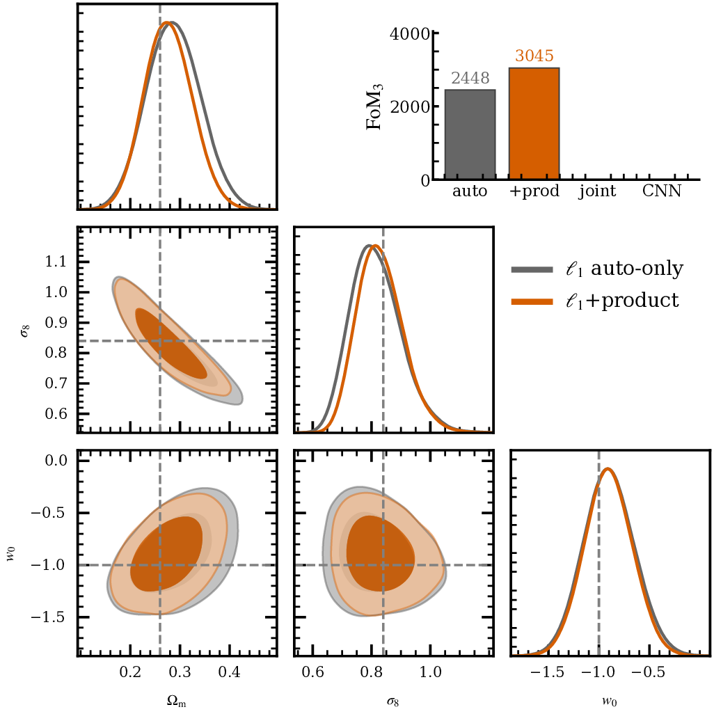
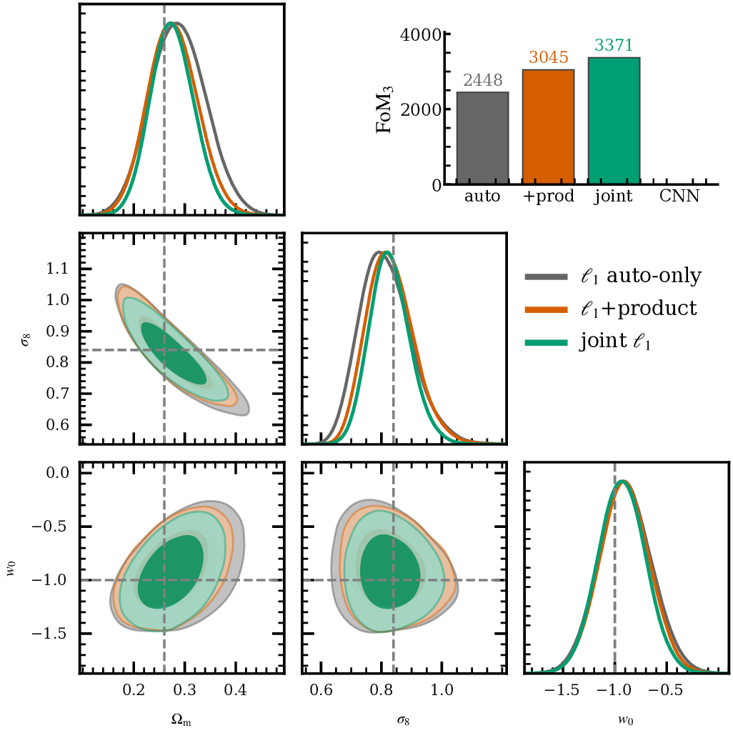
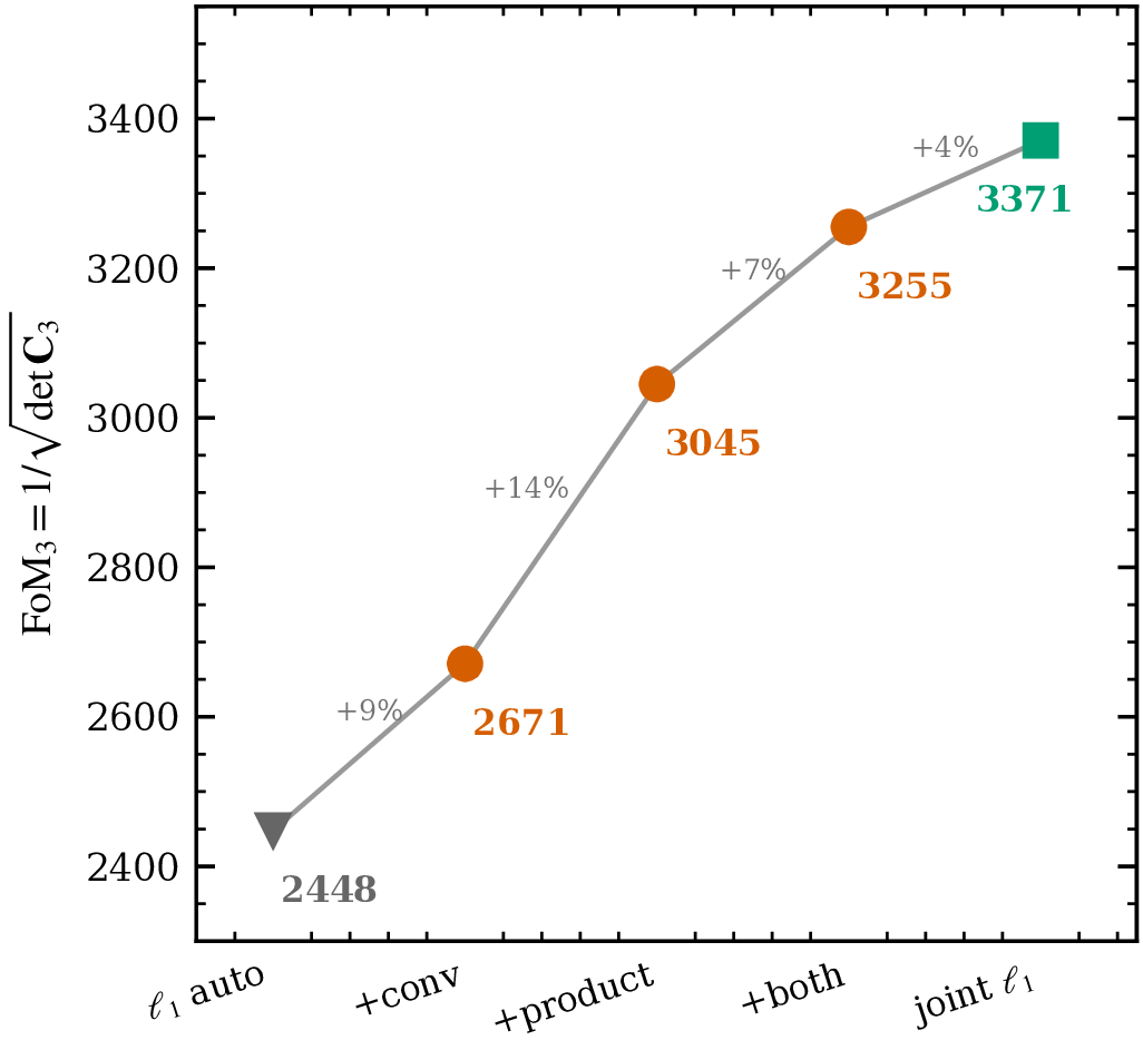
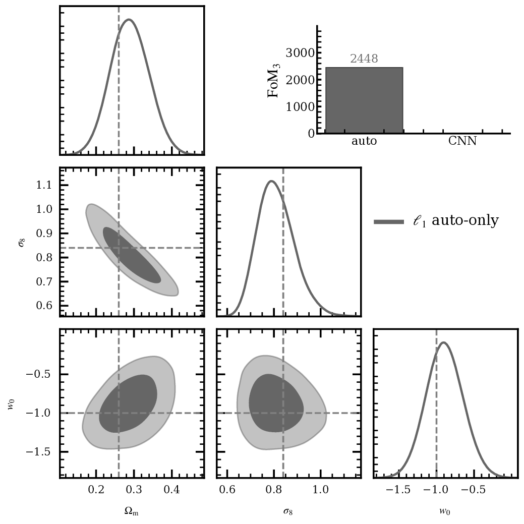
three-parameter figure of merit, matched pipeline

one bin at a timeℓ1, auto-maps

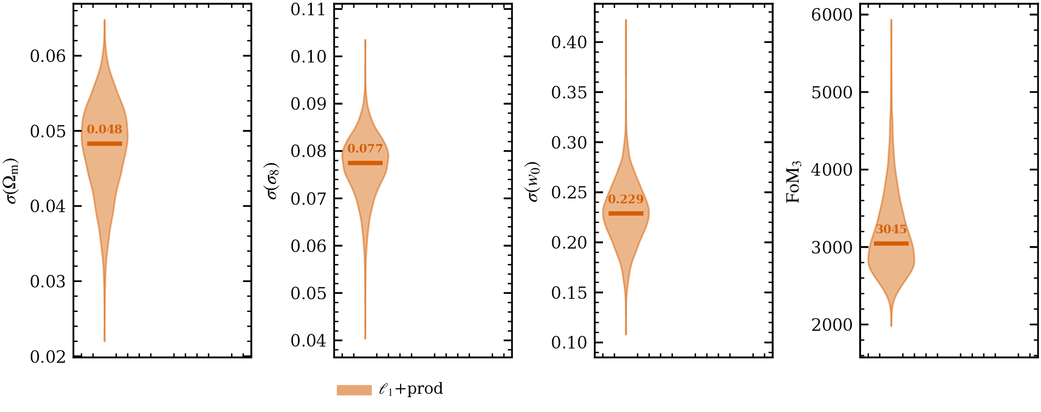
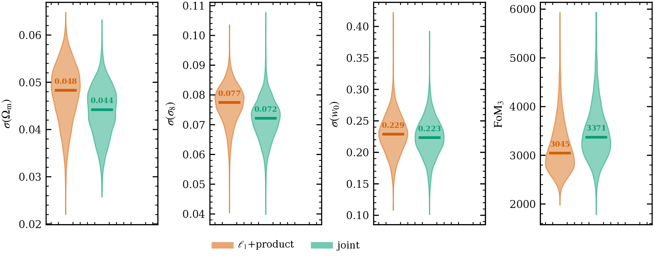
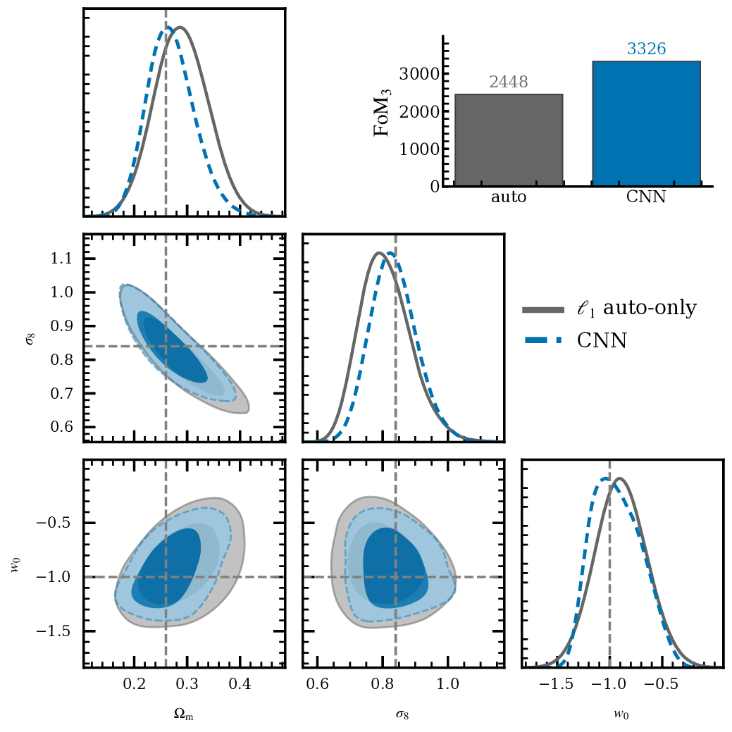
2448

+ a derived field per pairℓ1 + product cross-maps

3045

each pair's full 2-D distributionjoint ℓ1-norm, new

3371

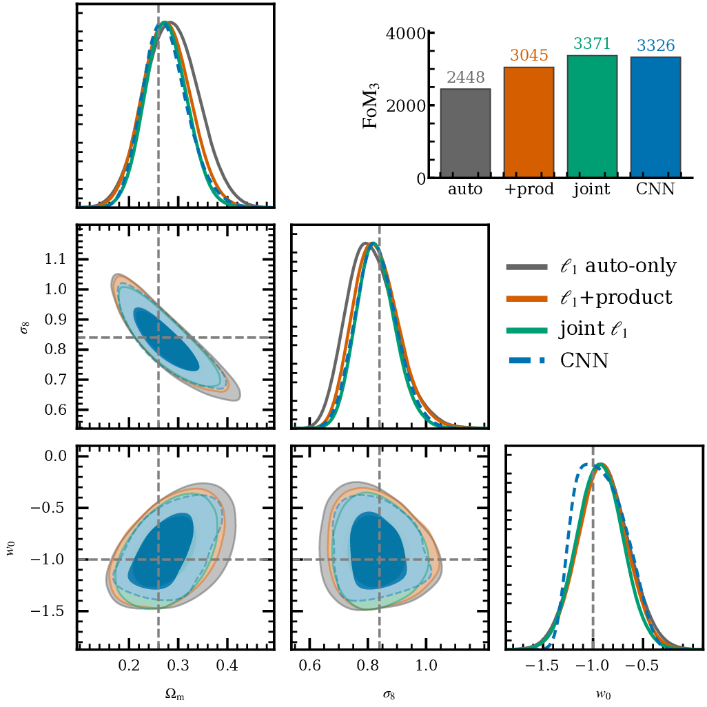
all four channels at onceCNN, VMIM-trained

3326

↑ the ceiling, a compressor trained to be optimal

per-mock distributions of the marginal uncertainties and the figure of merit for the l1 plus product, joint l1 and CNN summaries; the medians coincide — a tie on every parameter, over 9,000 mock observations — not a figure-of-merit artefact

Q2 Given the same constraining power, everything else decides

constraining power joint ℓ1-norm 3371 ≈ CNN 3326

fixed — the ℓ1-norm

Fixed before any simulation is seen
No training, nothing to overtrain
Survives a change of survey or forward model
Open to inspection, scale by scale
Analytically predictable on large scales

learned — the compressor

Retrained for every change of configuration
Seed-to-seed scatter
Ten coordinates with no meaning to inspect
Cannot tell physics from simulator artefacts

The compressor keeps one advantage: it reads the bins jointly for free. Which matters next.

§0 We are all optimizing statistics; the two-point camp still does not trust the contours

🧐

the 2-point camp

"I don't believe any of your contours."

what would make HOS flagship-grade?

blinding
robust covariance
emulators
systematics
analytical cross-checks
non-Gaussian likelihood
method limits
null / validation tests
simplicity

Part 1 of 2

Do baryons break HOS?

Baryonic feedback, the wavelet ℓ1-norm, and the BNT transform.

§1 Stage IV is no longer statistics-limited, it is systematics-limited

to trust a statistic

Before we trust any summary statistic, we have to quantify how each systematic affects it, and at the contour level (the inferred parameters).

Illustris: baryonic feedback reshaping the cosmic web

the systematic at hand

Baryonic feedback (AGN, supernovae) suppresses matter on small scales, mimicking cosmological signal and biasing inference, exactly where the constraining power lives and where the feedback models disagree most.

core questions

How does unmodeled baryonic feedback bias our non-Gaussian statistics?
After safe scale cuts, do HOS still outperform the power spectrum?

Part 2 of 2

Learned vs analytical,
and can we trust it?

The analytical ℓ1-norm vs a learned CNN, calibration, and the answer to the BNT puzzle.

§2 Part 2: learned summaries, and the BNT cliffhanger

the question How much better are "optimal", learned summaries than our hand-built summary statistics?

what is a learned summary?

A neural network that compresses the κ map directly into a few numbers, instead of a hand-designed statistic
Trained with VMIM to keep the cosmological information: the "optimal learned compressor"

and, left over from Part 1 ...and what the hell is going on with BNT?

Training a neural summary I: regression (MSE)

simulator

$\theta\sim$ prior

→

map $x$

→

network

$f_\phi$

→

estimate

$\hat\theta$

\[\mathcal{L}=\mathbb{E}\,\big\lVert\,\theta-f_\phi(x)\,\big\rVert^{2}\]

parameter space $\theta$

§2 Can we trust it? Every arm passes the same TARP + SBC tests reasonably

TARP-DRP expected coverage against credibility level, every arm arriving in turn and every one lying on the diagonal — TARP-DRP coverage: on the diagonal

SBC rank densities for every arm and every parameter, flat within the band, in both the standard and the nulled frame — SBC ranks: flat within the band, standard frame and nulled (dashed)

SBC ranks: flat within the band, standard frame and nulled (dashed)

tight is not the same as correct

Both arms pass the same battery: varied-θ TARP-DRP coverage + SBC rank uniformity
The constraining power is real

Same information, a different frame: why BNT collapses the ℓ1-norm but not the CNN

the point cloud (all the information) never moves

lensing kernels q(z)

Signal & noise under BNT: who can read it

noise covariance

What survives BNT: the 2-point rule

§2 The analytical statistic ties it — and it is the safer instrument

the benefit

a tie

Joint ℓ1 3371, CNN 3326, both calibrated. The optimised network buys no measurable constraining power.

the cost

extensive architecture and hyperparameter search
a very large dataset (899 cosmologies, 3.2×10⁵ patches); VMIM needs the scale or it biases
unphysical-information traps (patch geometry, map-mean / mass-sheet mode, 20° projection features) that tighten contours dishonestly
and these largely escape TARP and SBC: the contours look calibrated and are still wrong

the thumb on the scale

ℓ1 is simple, interpretable, inspectable; CNNs are powerful but treacherous
Where the CNN earns its keep: BNT, the channel-mixing win
So the question is not whether the network wins, but what the cost and the risk are buying

§3 Do baryons break HOS? No.

Part 1, baryons Usable non-Gaussian information persists on baryon-safe scales (the ℓ1-norm beats P(k) ×1.8 at Stage IV, ×2.6 at full sky), cleaned by a single scale cut.

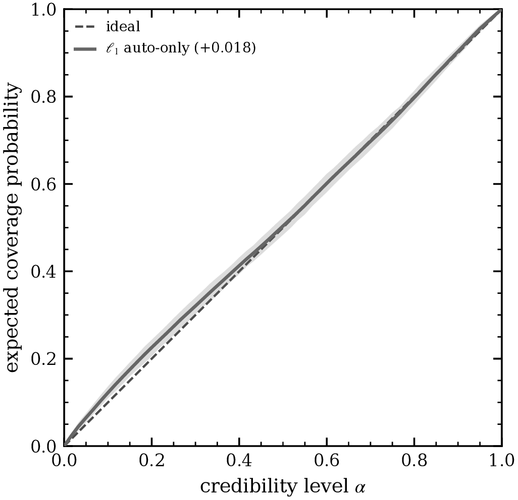
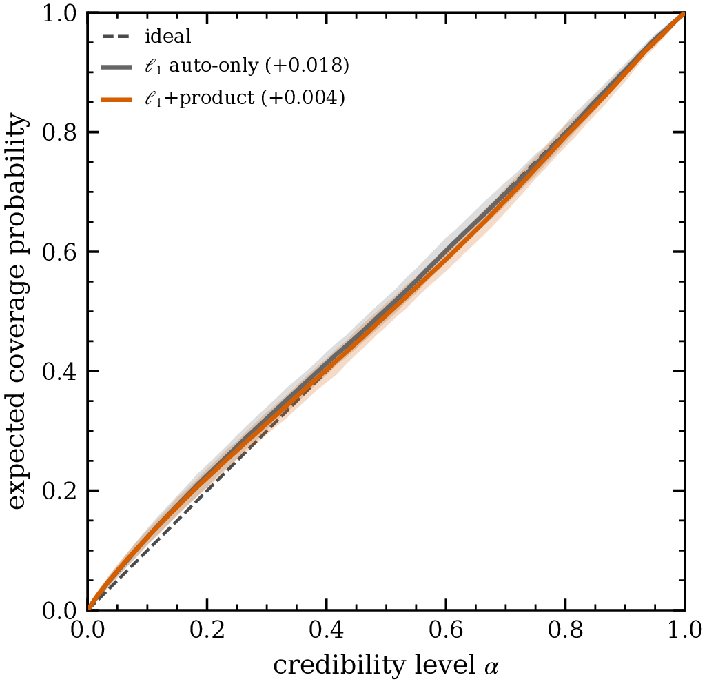
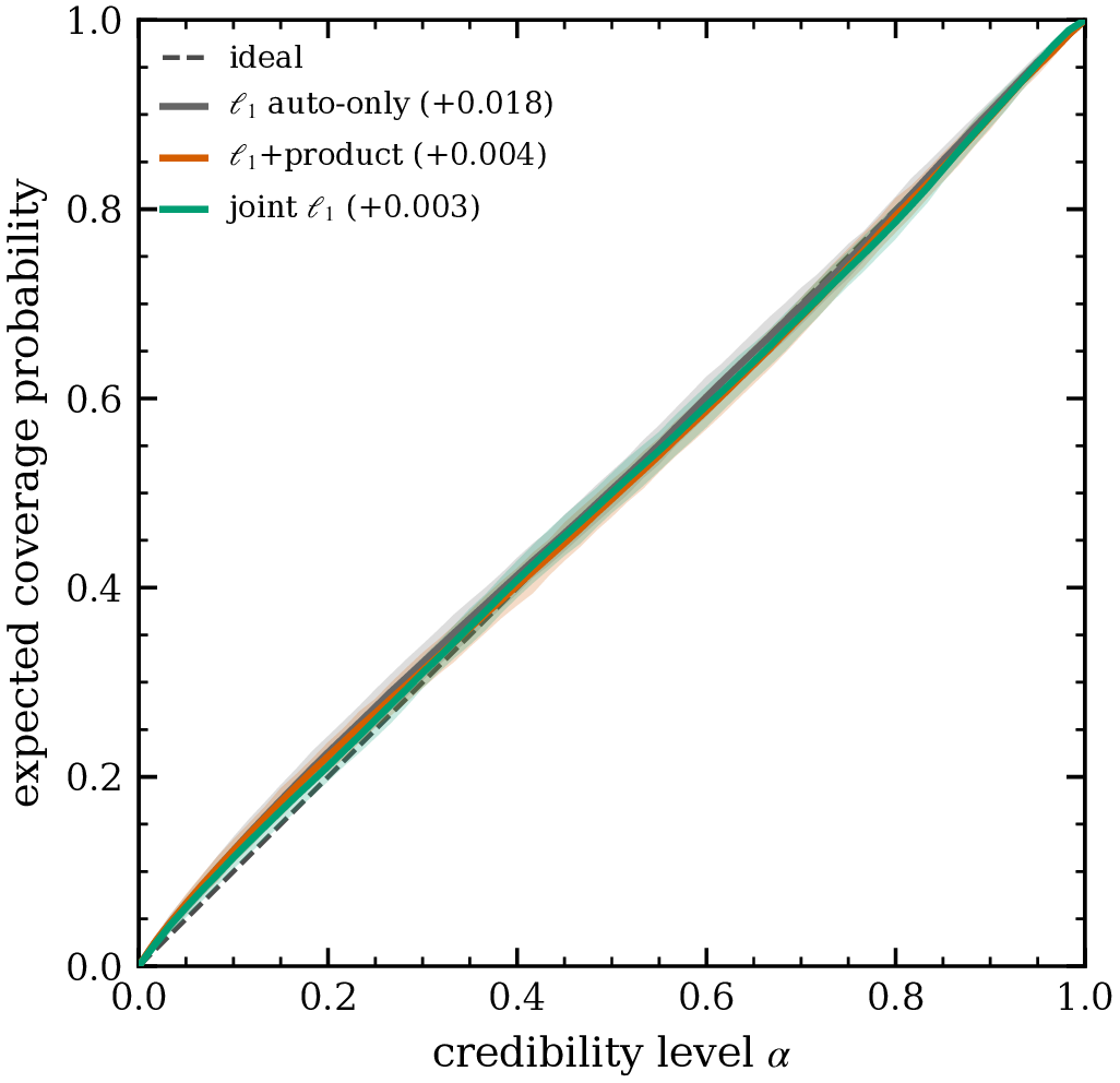
Part 2, learned vs analytical Read the bins jointly and the hand-built ℓ1-norm matches the optimal learned summary — 3371 against 3326, a tie, both calibrated.

BNT The apparent BNT break is a frame artifact: what survives tracks how jointly the summary reads the bins — 0.16, 0.24, 0.72, 0.96.

the bigger question And can we trust higher-order weak lensing? Getting there...

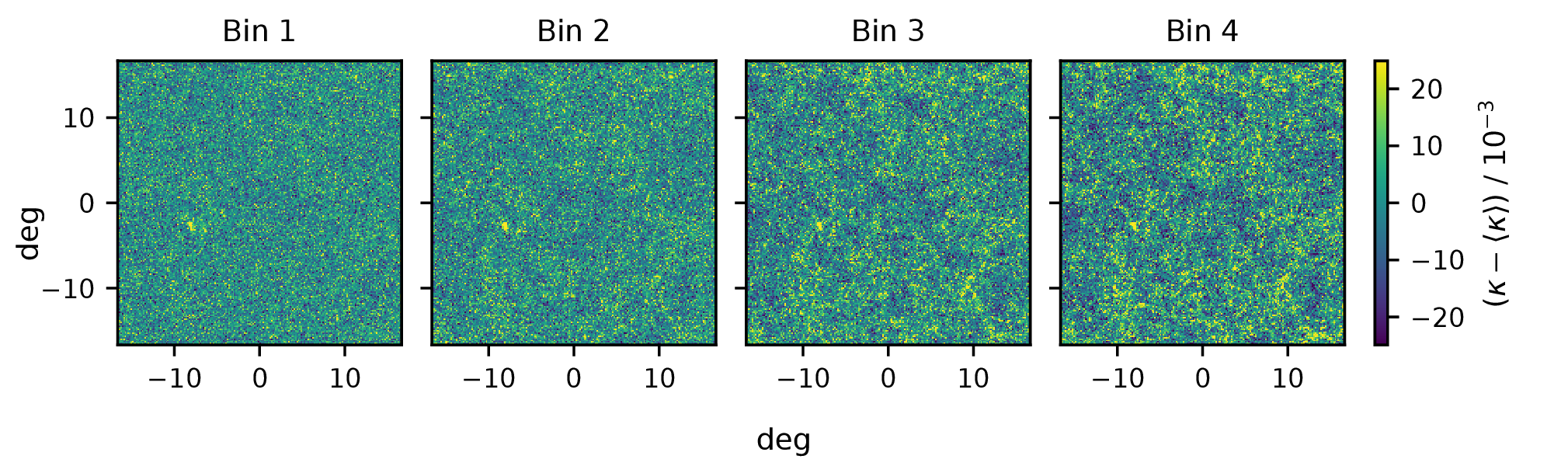
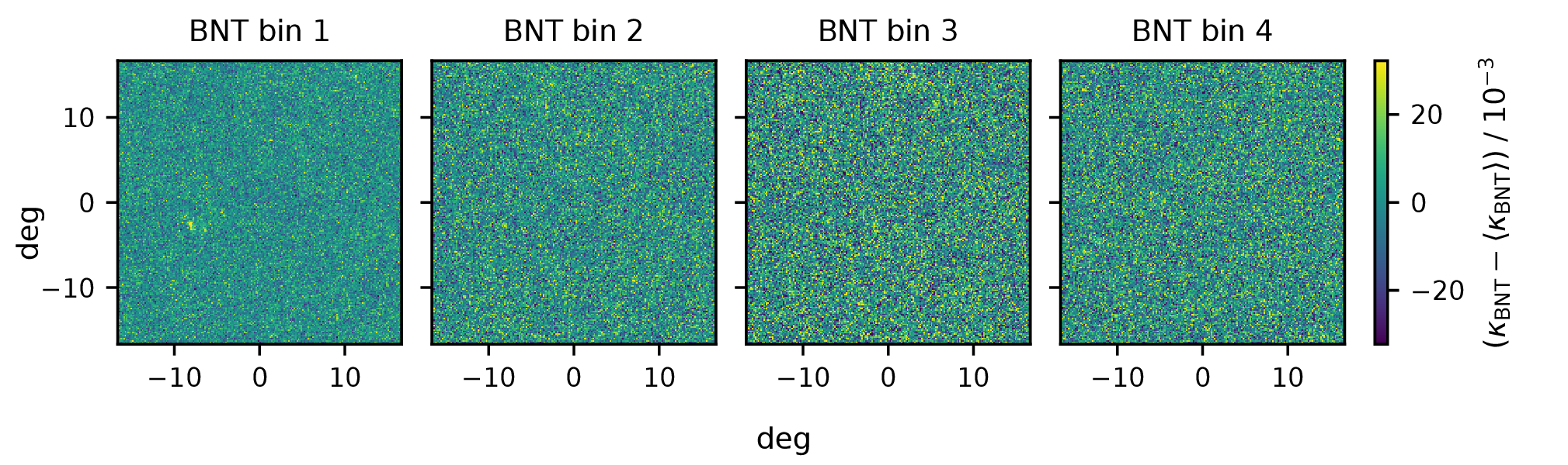
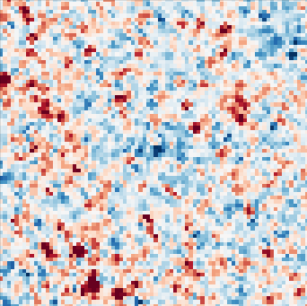
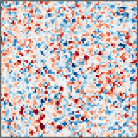
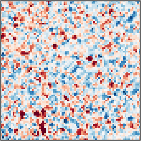
§1 You can see it in the maps: BNT trades deep signal for amplified, correlated noise

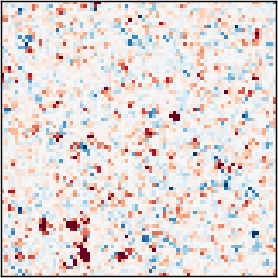
noisy tomographic maps before BNT — before BNT

noisy maps after BNT, visibly degraded SNR — after BNT: the SNR collapses

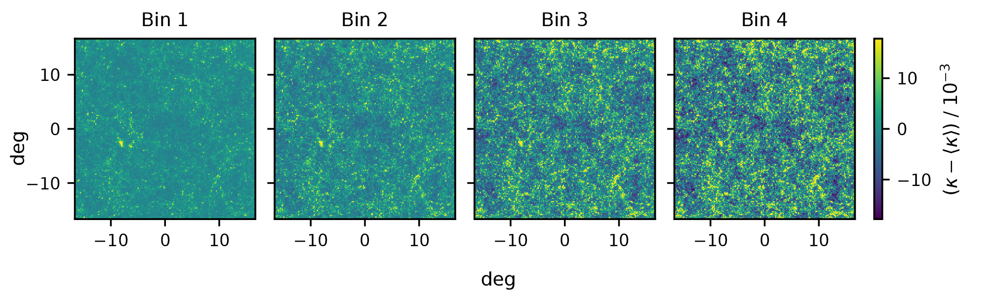
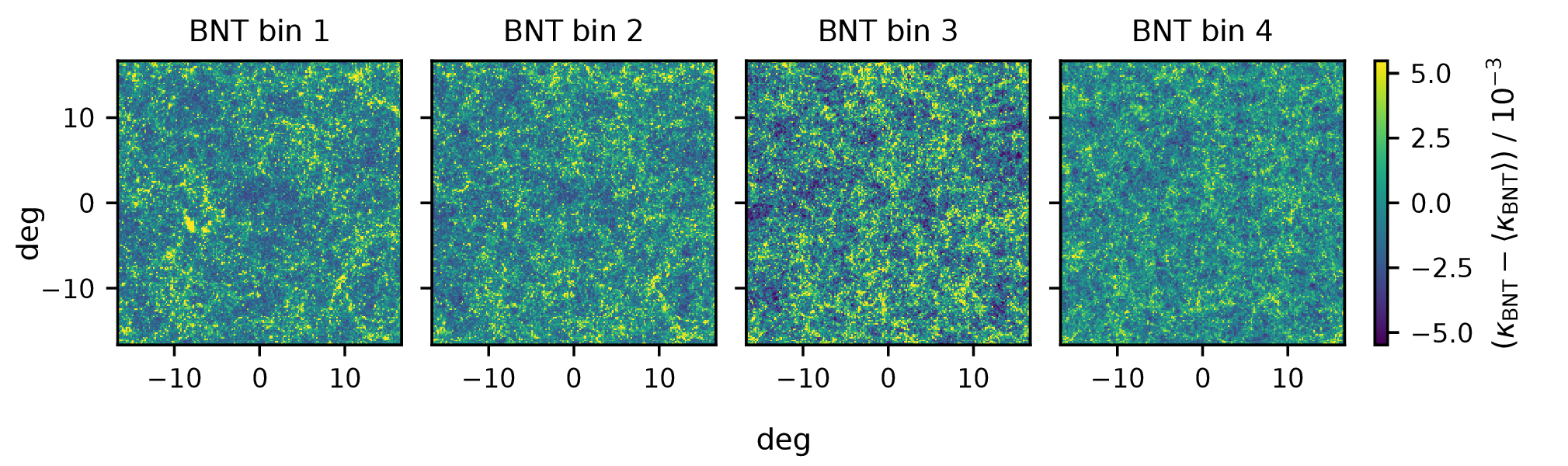
§1 The same maps, noiseless: BNT cleanly redistributes the signal

noiseless tomographic maps before BNT — before BNT (noiseless)

noiseless maps after BNT — after BNT (noiseless)

Without shape noise, BNT is a clean, invertible redistribution of the signal (the deep common mode becomes one shallow map plus thin slices). The contour inflation comes from the correlated noise it introduces, not from any lost signal.

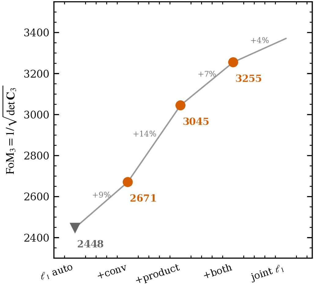
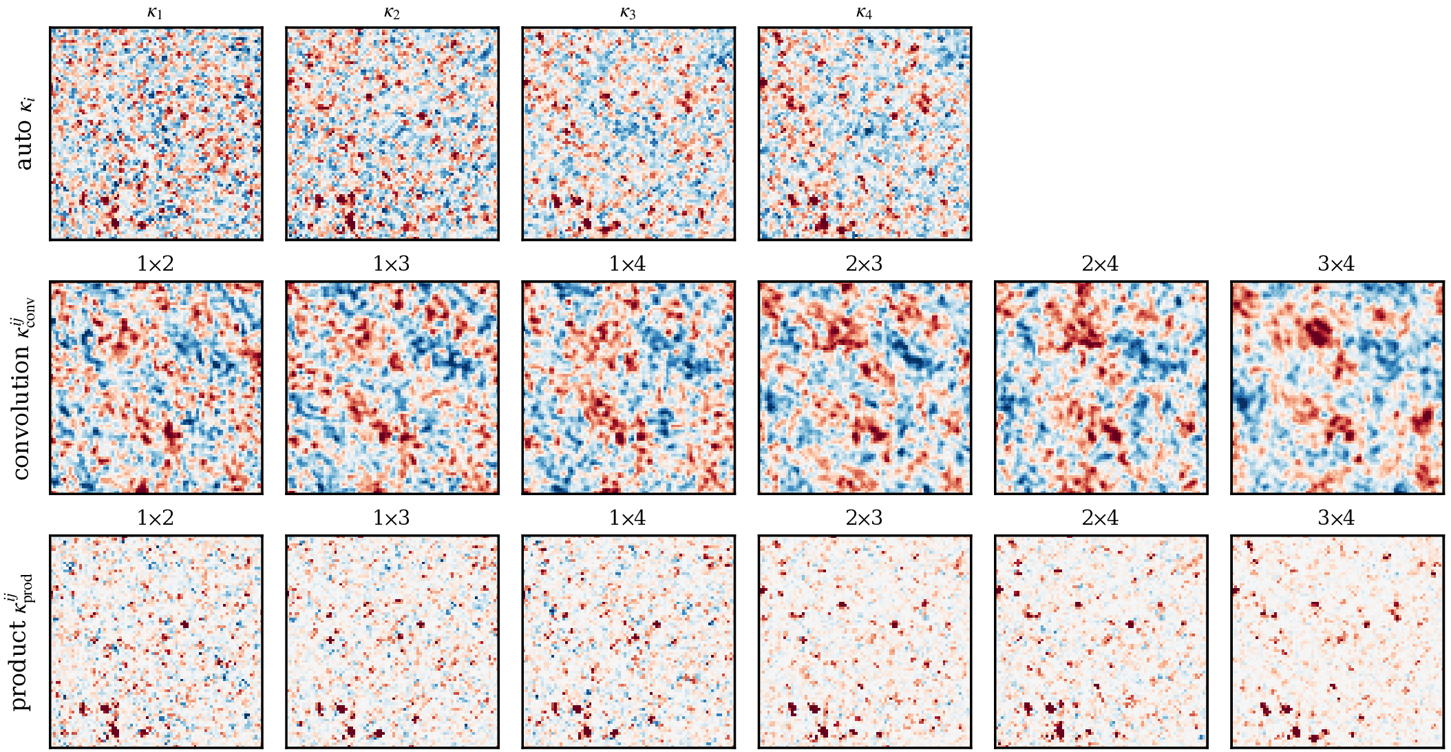
§2 Where the cross-bin information lives: the κ_iκ_j product buys +24%, and reading each pair jointly buys the rest

the completeness ladder in figure of merit: auto 2448, plus convolution 2671, plus product 3045, both 3255, joint l1 3371

add the cross-bin physics carefully

Product κ_iκ_j (= ξ_ij): +24% over auto-only
A convolution buys +9%, and is sensitive to the training realisation
2448 → 2671 → 3045 → 3255, and the joint ℓ1 closes it at 3371

A full-sphere cross construction inflates this, but its channels carry 12–20% of their variance at ℓ < 18 against 0.4–1% for the autos. That is leakage. We use only the physically buildable flat-sky arms.

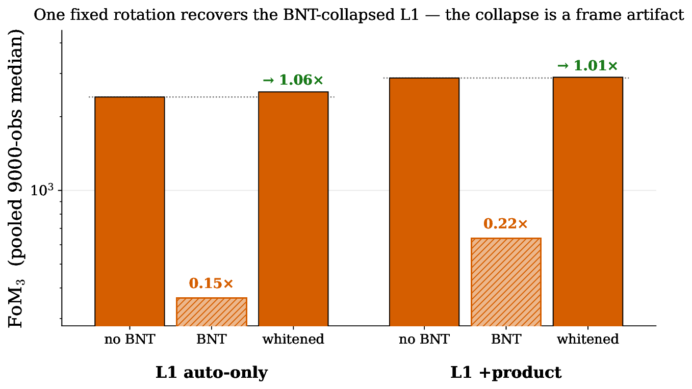
§2 The clincher: a frame artifact, not lost information (one rotation recovers ℓ1, 1.06×) unpublished — not in Paper II

no-BNT, BNT collapsed, and whitened (recovered to 1.06x) per arm

the information was never lost

One fixed whitening rotation Q recovers the full no-BNT FoM3 for ℓ1 too (1.06×)
The collapse is a per-channel frame artifact: mix the bins, or re-rotate once
Confirms the intuition block; closes the Vinciguerra loop

Closes the Vinciguerra loop: their forecast said recovering the BNT SNR for HOS is "highly non-trivial"; here it is, in one fixed rotation. A frames result: a one-point statistic's information content is basis-dependent, and BNT is simply a poor frame for a per-channel statistic.

§3 One story: the optimal tomographic strategy (BNT becomes viable once the summary mixes bins)

per-bin l1 contours inflate under BNT — problem: the per-bin ℓ1 inflates under BNT

→

the channel-mixing CNN posterior is indistinguishable in the standard and the nulled frame — resolution: a summary that reads the bins jointly is unaffected

one escalating story about cross-bin information

P(k) → ℓ1 (much more, even on safe scales) → learned (a tie, both calibrated)
Per-bin statistics cannot access cross-bin info (break under BNT); a channel-mixing compressor can (BNT-lossless)
BNT becomes viable once the summary mixes bins

Forward-looking: a route to baryon-robust, non-Gaussian SBI that keeps BNT's clean per-bin scale cuts without the contour-inflation tax. A next step, not a finished end-to-end measurement.

backup Constraining power against survey area, all three statistics

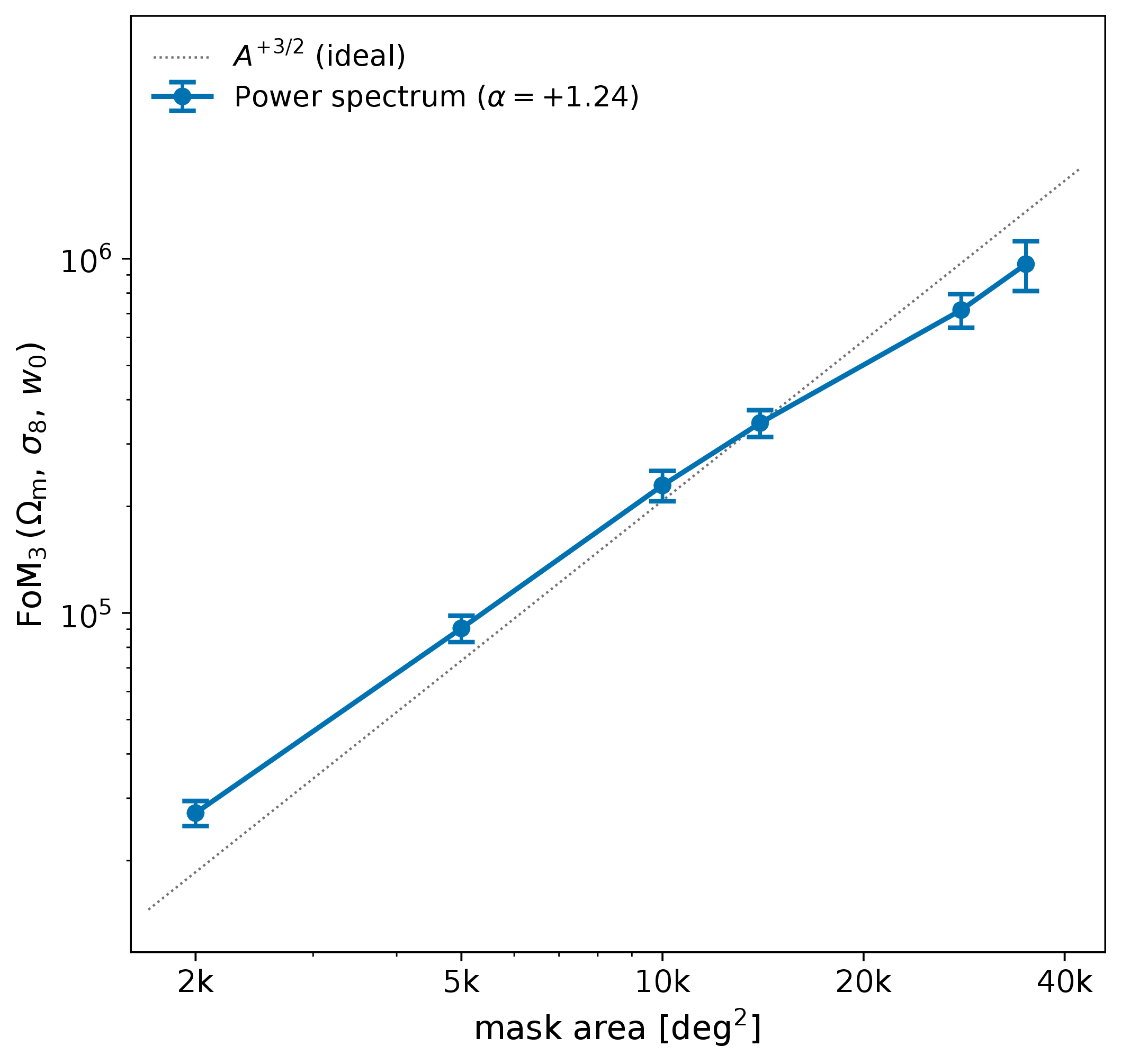
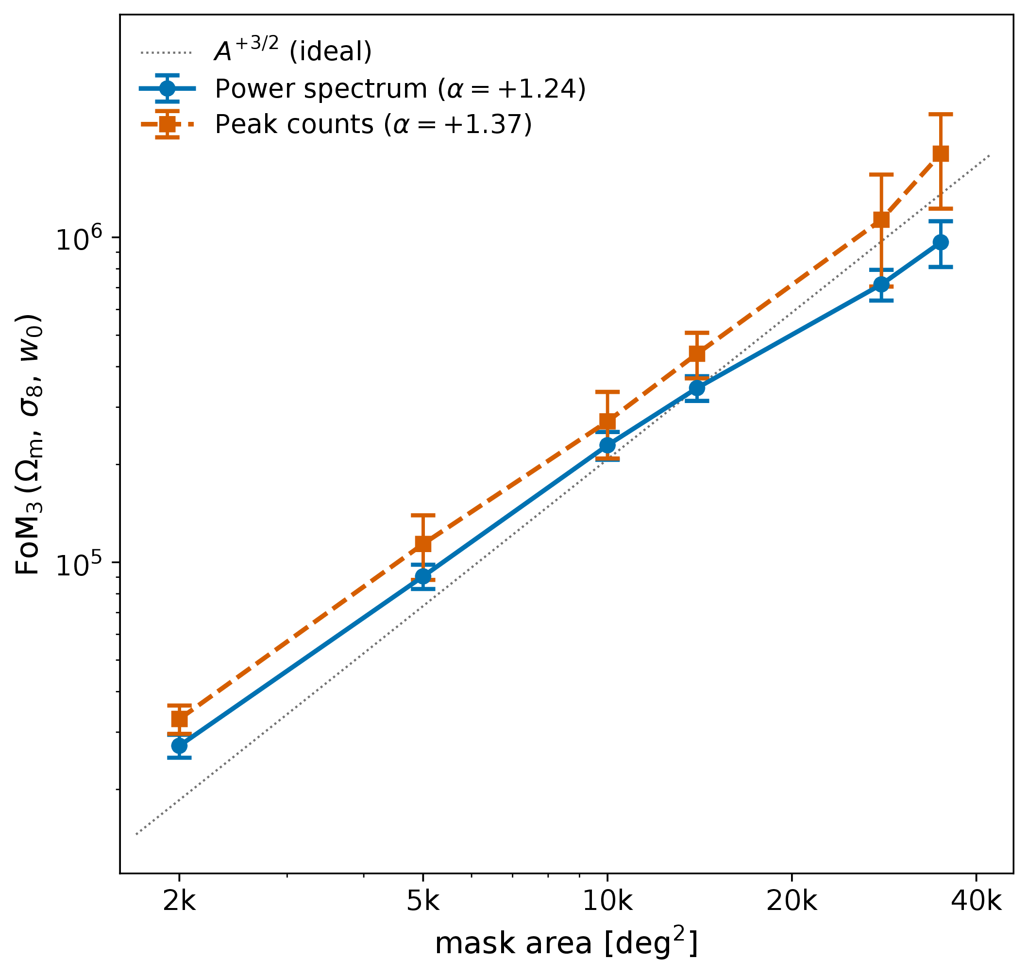
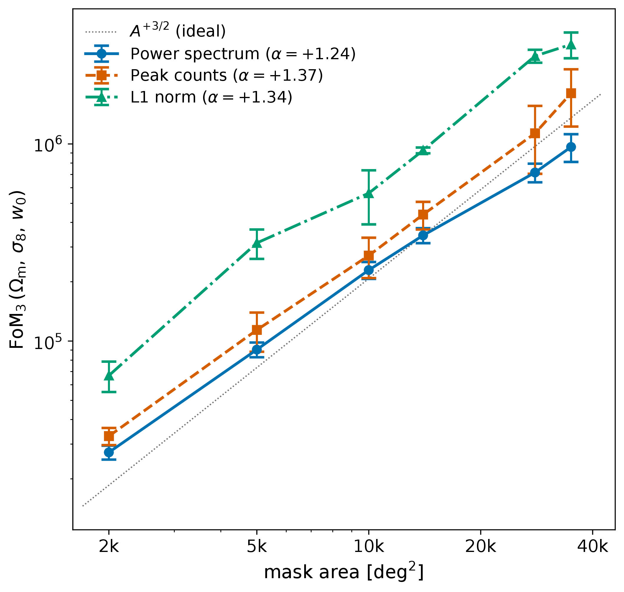
figure of merit against mask area for the power spectrum, peak counts and the l1-norm, each with its fitted power-law slope

On baryon-safe scales. Fitted slopes: power spectrum $+1.24$, peaks $+1.37$, $\ell_1$-norm $+1.34$, against the ideal $A^{+3/2}$.

backup The starlet band responses in multipole

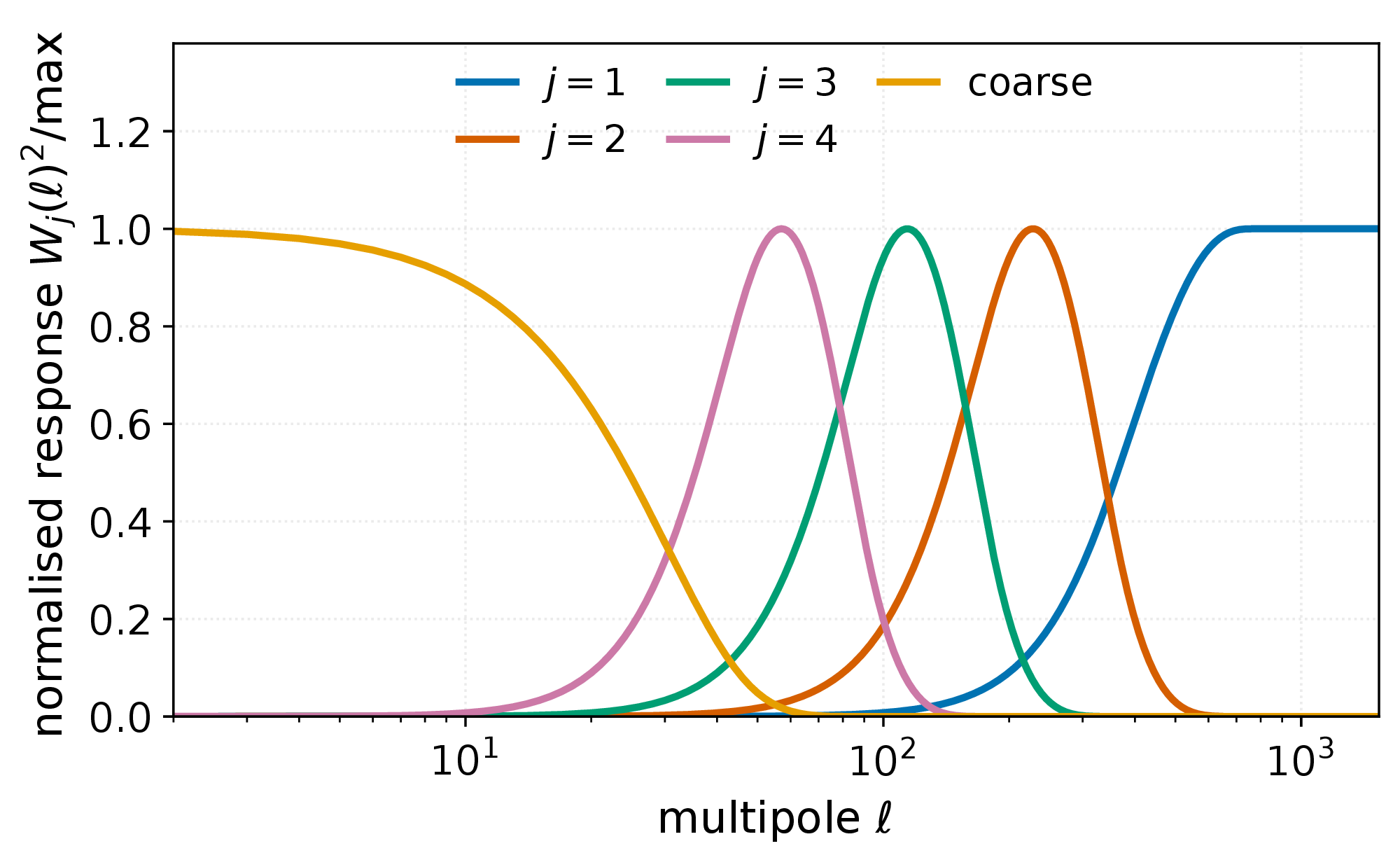
normalised squared response of each starlet band against multipole, the four dyadic bands plus the coarse scale

This is what "drop $j=1$" removes: the highest-frequency band, everything above $\ell \approx 500$. The other bands are untouched, at every survey area.

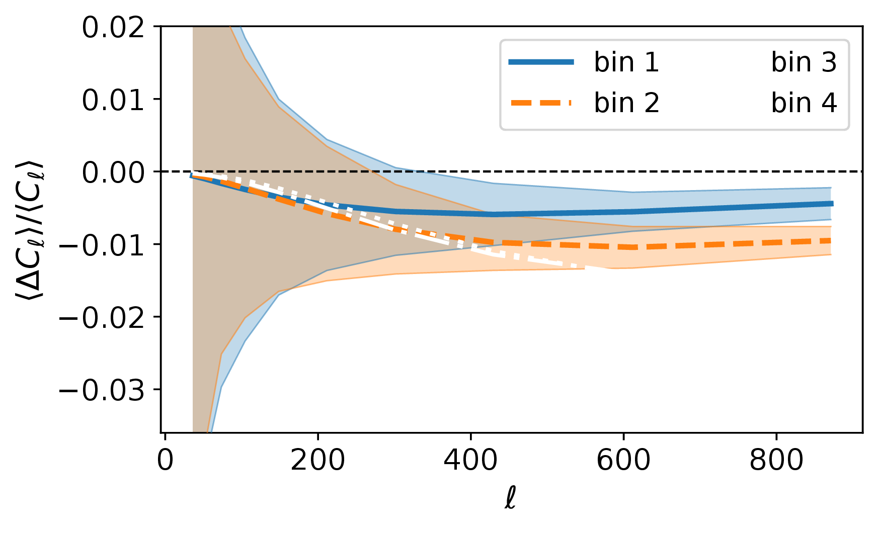
backup BNT on the power spectrum: the bin-specific cut is worth ×1.4

power-spectrum posteriors at 14,000 square degrees: the standard basis with a global lmax of 460 against the BNT basis cut only in the first transformed bin

Baryon sensitivity localises to the first transformed bin, so the cut goes there alone and bins 2–4 keep $\ell_{\rm max} \approx 1024$: 92 of 120 bandpowers retained against 50 for the global cut. σ(Ω_m) −14%, σ(σ₈) −19%.

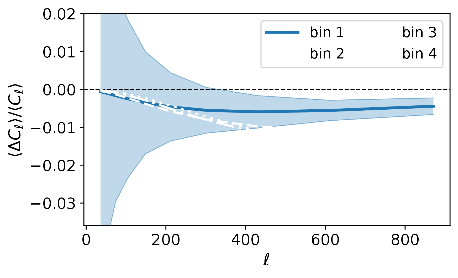
backup Baryonic suppression of the tomographic power spectra

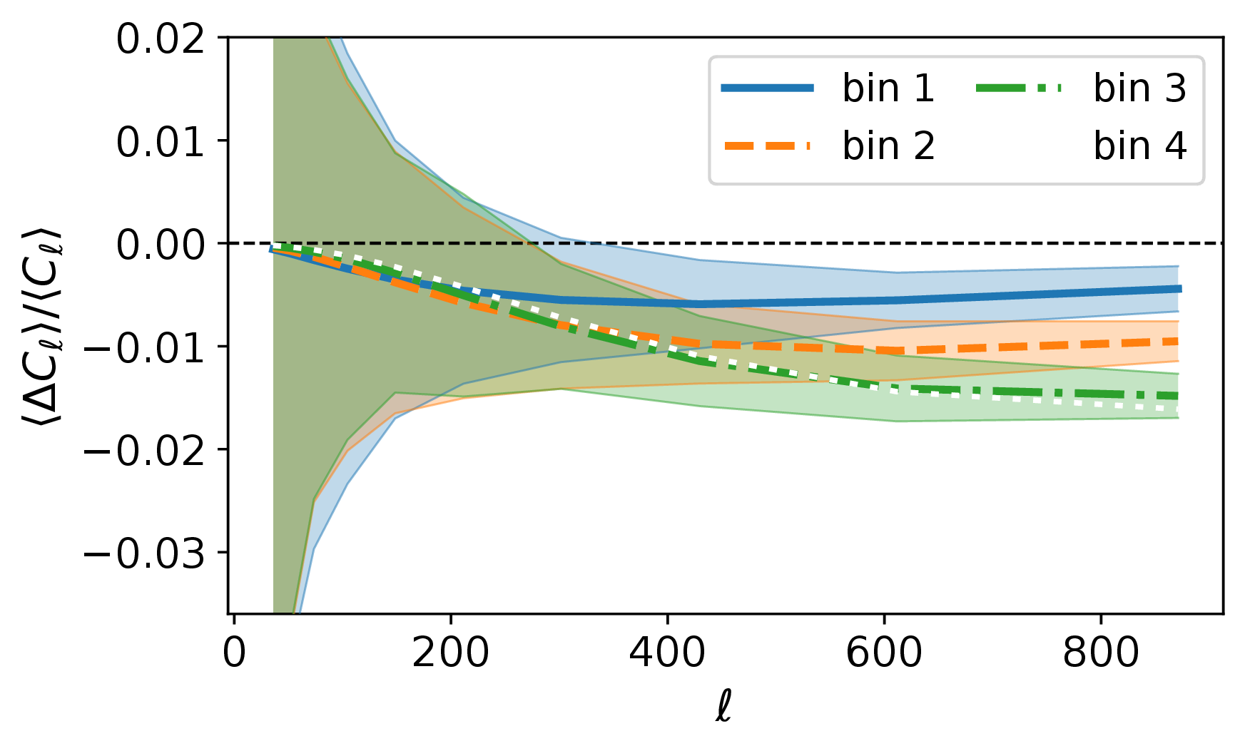
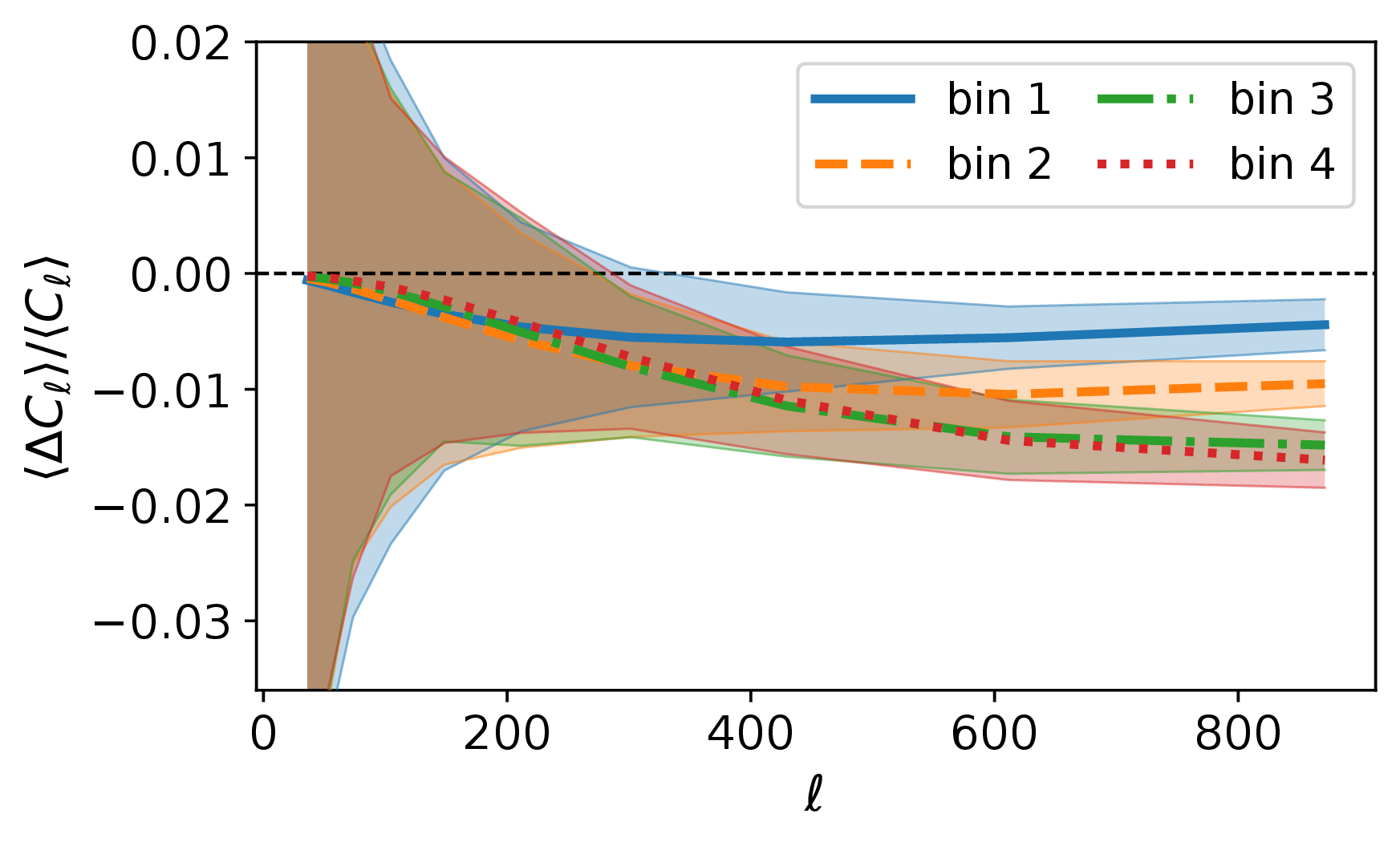
$fractional change in the tomographic angular power spectra from baryonification, one curve per source bin$

Reaches ≈1.5% by $\ell \approx 1000$. The apparent "high-z bins are worse" ordering is a noise artefact — the noise power dominates the denominator at low z. On noiseless maps the ordering inverts to the physically expected one.

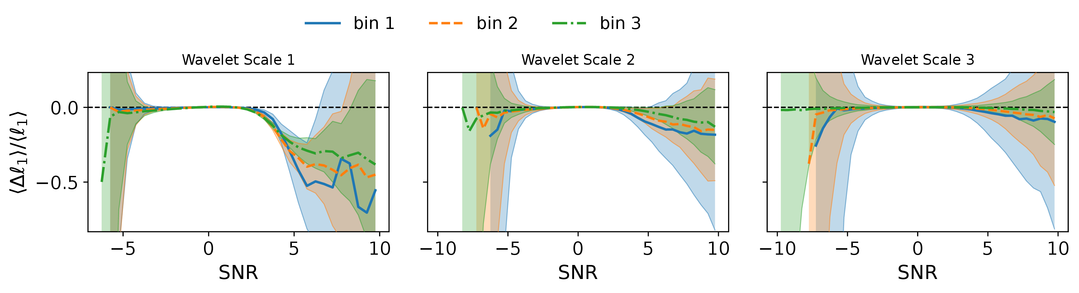
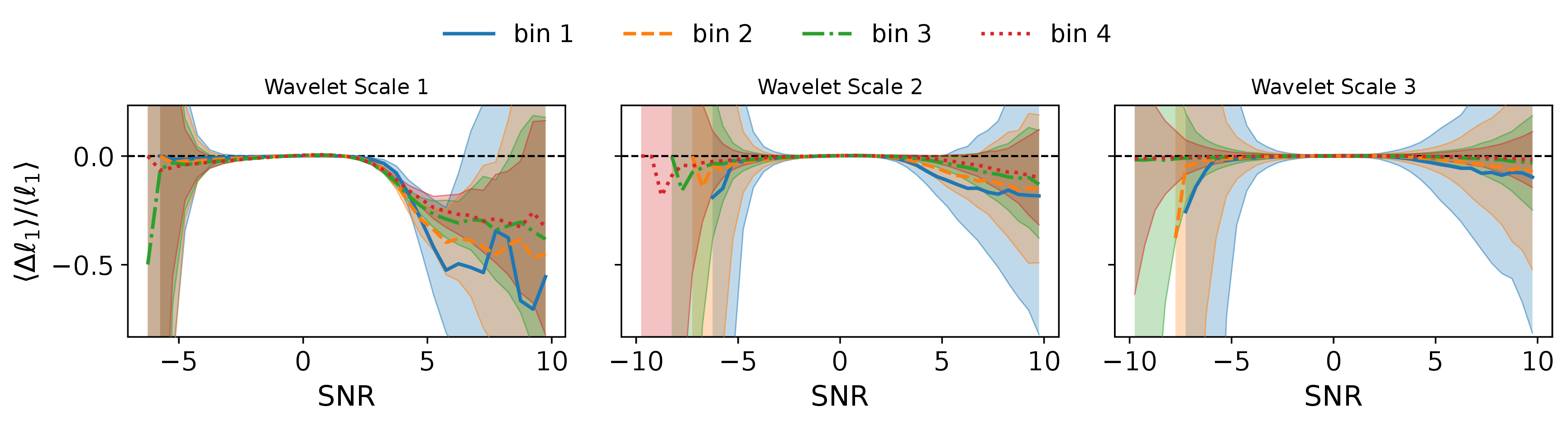
backup Baryonic response of the ℓ1-norm, scale by scale

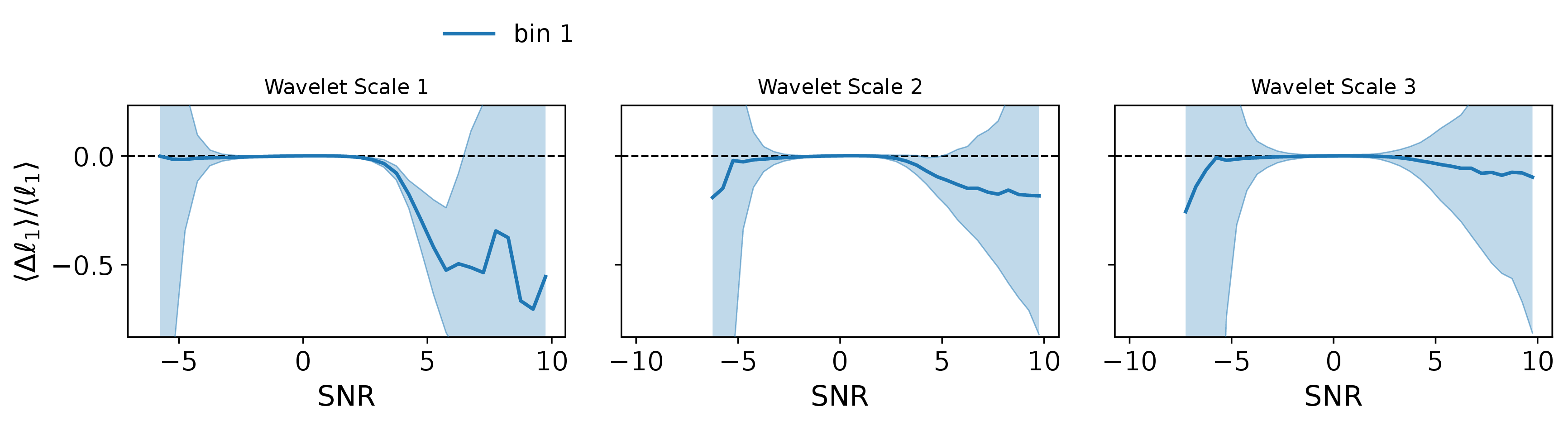
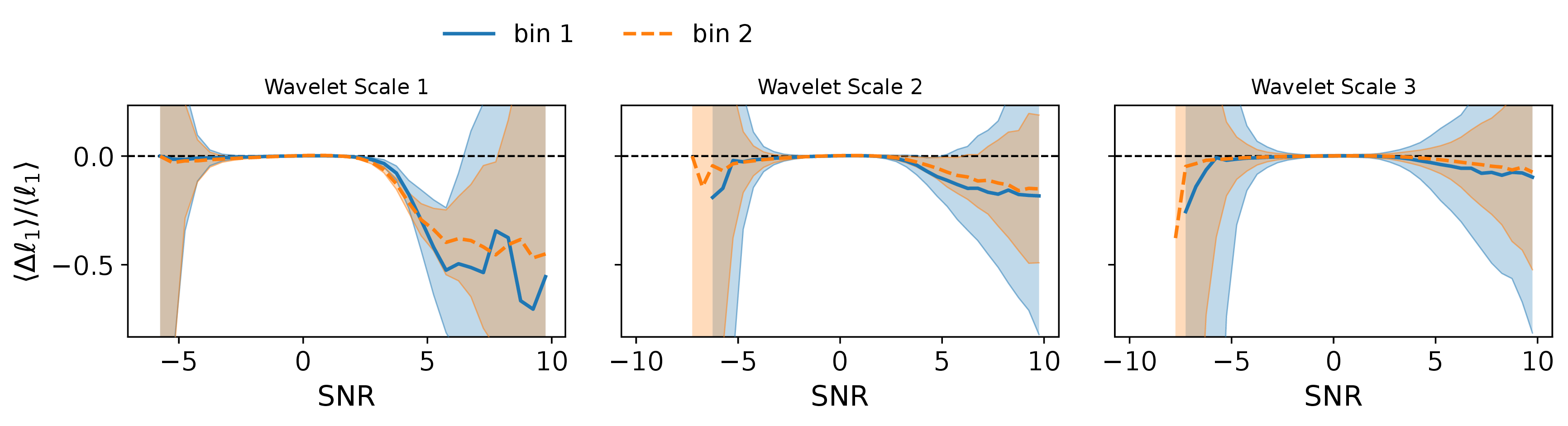
$fractional change in the starlet l1-norm from baryonification, per wavelet scale and signal-to-noise bin, one curve per source bin$

Concentrated in the positive SNR tail, and vanishing in the noise-dominated bulk ($|\nu| \lesssim 2.5$) — which is why an SNR-space cut is available to higher-order statistics and not to the power spectrum. Left to future work in the paper.

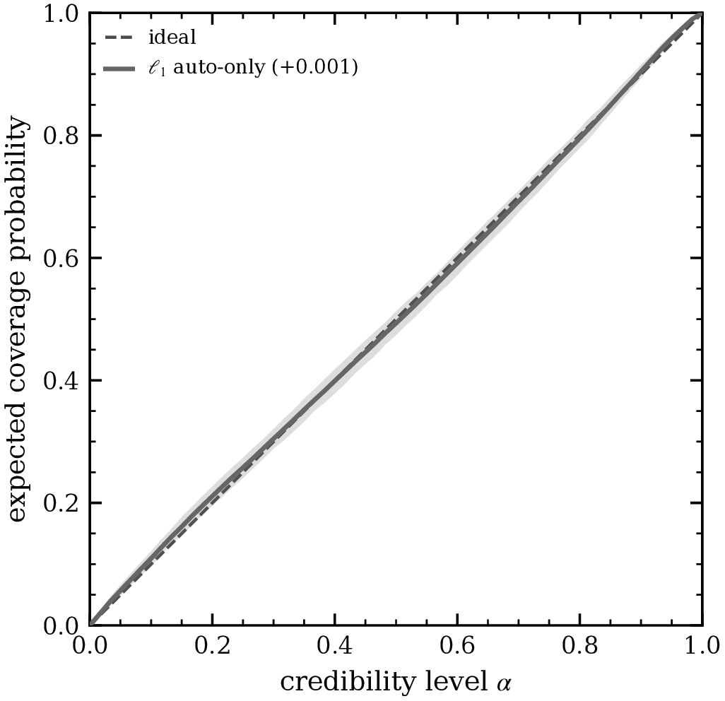
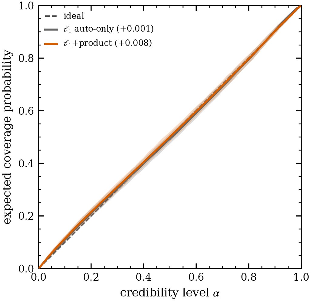
backup Coverage in the nulled frame: every arm still passes

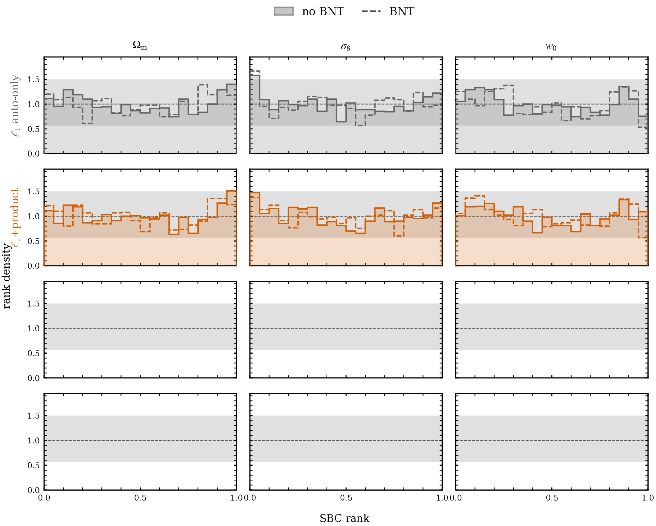
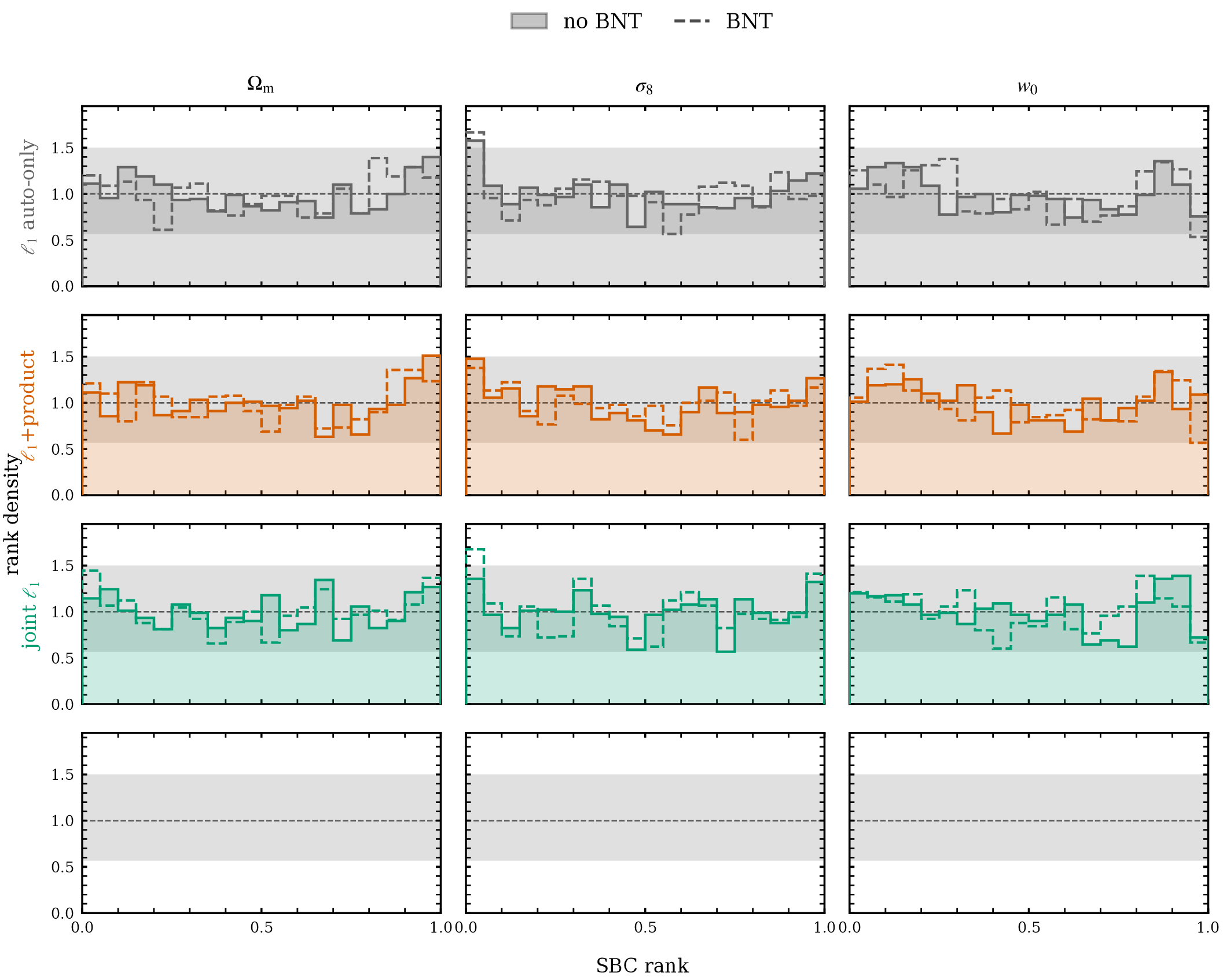
TARP-DRP coverage in the BNT basis, every arm on the diagonal

The collapse is calibrated. The wide contours are an honest report of a real loss in that representation, not over-confidence — which is what makes the retention ladder a statement about information rather than about a broken fit.

backup Where the ℓ1-norm’s constraining power sits

relative Fisher information of the auto starlet l1-norm per wavelet scale and signal-to-noise bin, for each of the three parameters

Intermediate scales ($j = 2$–3, tens of arcminutes) and moderate signal-to-noise ($|\nu| \approx 1$–2) — mildly non-linear structure, not the rare extreme peaks. Dovetails with Paper I: drop $j=1$ and you keep most of it.

backup The ℓ1-norm across cosmologies

starlet l1-norm data vectors coloured by sigma-8, per wavelet scale and tomographic bin

Coloured by $\sigma_8$. The statistic responds smoothly and monotonically across the prior — no training, no emulator, and the dependence is visible by eye.

backup The data: flat-sky tomographic patches

example 10 degree gnomonic convergence patches across the four tomographic bins, noiseless and noisy

10°×10° gnomonic patches, 80×80 px (7.5′/px), $|b| < 75^{\circ}$. 180 patches per realisation × 50 noise realisations = 9,000 mock observations. Patch size chosen at 10° because gnomonic corner distortion falls from 6.3% at 20° to 1.5% at 10°.

backup The tie, per mock rather than at the median

per-mock distributions of the three marginal uncertainties and the figure of merit, for the l1 plus product, joint l1 and CNN arms

σ(Ω_m), σ(σ₈), σ(w₀) and FoM₃ across 9,000 mocks — medians 3045, 3371, 3326

The answer to “FoM₃ is fragile in a degenerate parameter space”: the marginals are quoted alongside it, and this is the population rather than a point. The ± on the medians is the spread over three independently trained compressors, the dominant source of run-to-run variability.

§2 The channel-mixing CNN does not notice the transform at all (0.96×)

the CNN posterior in the standard and the nulled frame, the two contours lying on top of each other

same maps, same transform, no cost Feeding the network the nulled maps gives the same first layer with kernels KB, so “undo the nulling” is one configuration of the first layer — available before any non-linearity, at no capacity cost. The 4% shortfall is an optimisation residual, not lost information.

§1 But could we do better than that? Weak lensing tomography

the source galaxies as tomographic convergence maps, one per redshift bin

Credit: Justine Zeghal