Fast likelihood-free inference in the LSS Stage IV era

G. Franco-Abellan, G. Canas-Herrera, M. Martinelli, O. Savchenko, D. Sciotti, and C. Wenigera

Andreas Tersenov

IA-FORTH Journal Club

slides at andreastersenov.github.io/talks/AstroML_JC_Mar24/

the $\Lambda$CDM view of the Universe

How does "standard" inference work?

Given data to analyze, $x$, that was generated through a model/random process → develop the likelihood, a model of the data generation process that describes the probability of the data given some parameters $\theta$ $$ p(x|\theta) $$ $$ \text{e.g.} \,\,\,\,p(x|\theta) = \mathcal{N}(\theta,1) = \frac{1}{\sqrt{2\pi}} \exp\left(-\frac{(x-\theta)^2}{2}\right) $$
Goal: perform inference on the parameters $\theta$ given the data $x$
Bayesian Inference: $$ p(\theta | x) = \frac{p(x|\theta) p(\theta)}{p(x)} $$
In typical statistics, we write down an analytic form for the likelihood.
Nice case: Can analytically derive posterior, confidence intervals, etc.
Not as nice: Can't analytically derive posterior, need to use sampling, e.g. MCMC

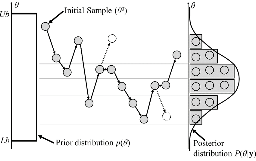
Metropolis-Hastings (MH) MCMC

Want to sample a (possibly un-normalized) distribution $p(x)$

Build a Markov Chain of samples $\{x_t\}$ → Transition to a new sample with a transition probability $q(x_{t+1}|x_{\text{t}})$ → The distribution of the samples converges to $p(x)$ as $t \to \infty$

Algorithm

Given current sample $x_t$
Draw proposal $x' \sim q(x'|x_t)$
Evaluate $a = \min \left[ 1 , \frac{p(x')}{p(x_t)} \right]$
Accept $x_{t+1} = x'$ with probability $a$
Stay at $x_{t+1} = x_t$ with probability $1-a$

The limits of traditional cosmological inference

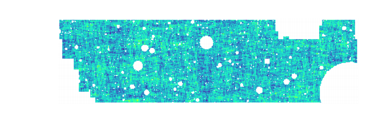
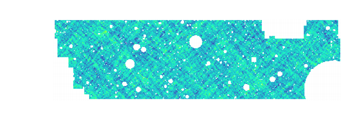
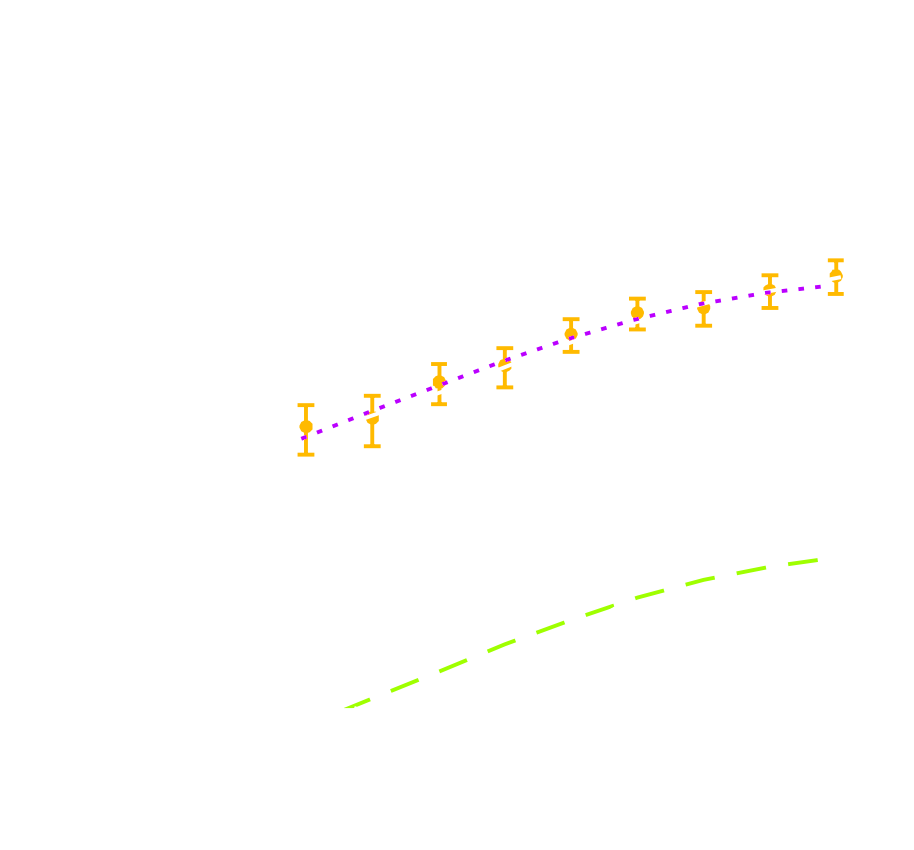
HSC cosmic shear power spectrum

HSC Y1 constraints on $(S_8, \Omega_m)$

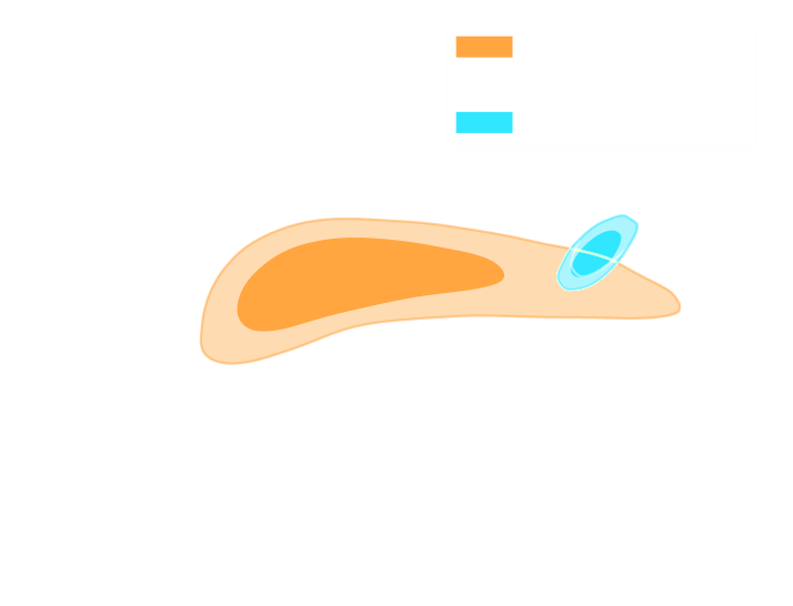
(Hikage et al. 2018)

Measure the ellipticity $\epsilon = \epsilon_i + \gamma$ of all galaxies
$\Longrightarrow$ Noisy tracer of the weak lensing shear $\gamma$

Compute summary statistics based on 2pt functions,
e.g. the power spectrum

Run an MCMC to recover a posterior on model parameters, using an analytic likelihood $$ p(\theta | x ) \propto \underbrace{p(x | \theta)}_{\mathrm{likelihood}} \ \underbrace{p(\theta)}_{\mathrm{prior}}$$

Main limitation: the need for an explicit likelihood

We can only compute from theory the likelihood for simple summary statistics and on large scales

$\Longrightarrow$ We are dismissing a significant fraction of the information!

Moreover, likelihood-based methods require sampling the full joint posterior $\Longrightarrow$ time to converge increases dramatically with the number of parameters.

Is there an alternative?

Simulation-Based Inference

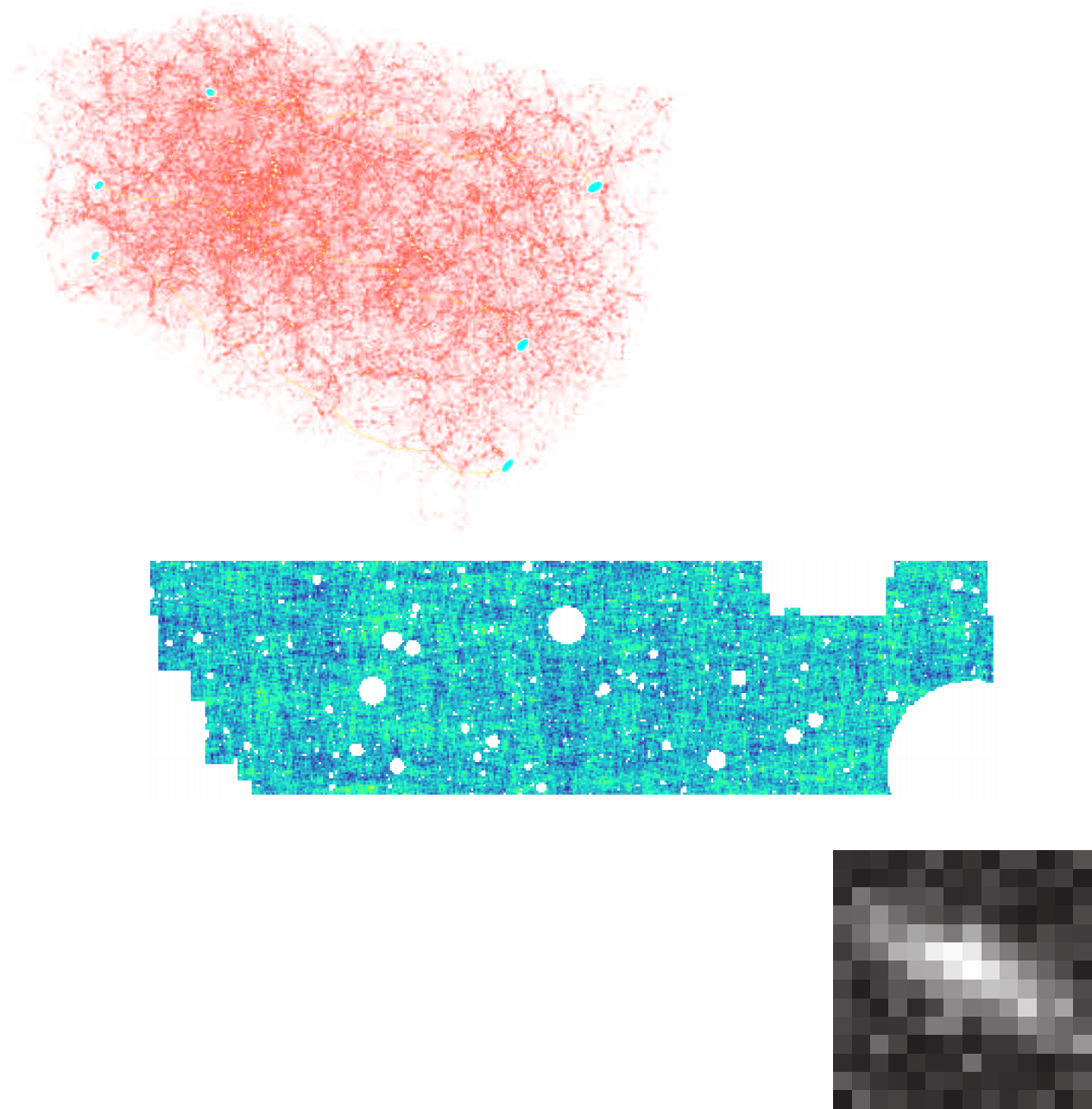
Instead of trying to analytically evaluate the likelihood of sub-optimal summary statistics, let us build a forward model of the full observables.
$\Longrightarrow$ The stochastic simulator becomes the physical model.

Allows us to sample observations given a set of parameters $\Longrightarrow$ this way, we can implicitly define $p(x|\theta)$.
Each component of the model is now tractable, but at the cost of a large number of latent variables.

Benefits of a forward modeling approach

Can fully exploit the information content of the data.
Easy to incorporate systematic effects.
Easy to combine multiple cosmological probes by joint simulations.

...so why is this not mainstream?

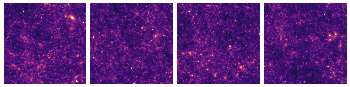
The Challenge of Simulation-Based Inference

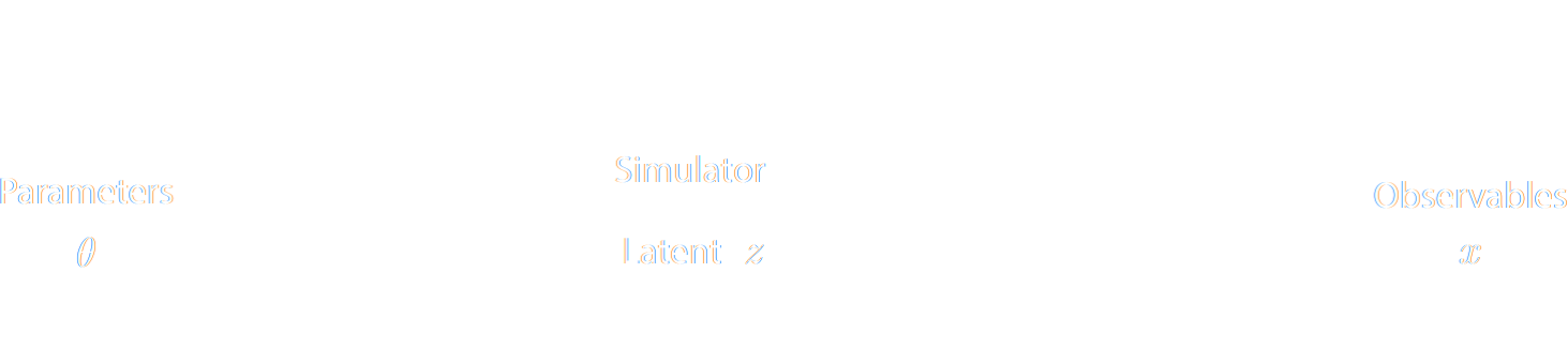
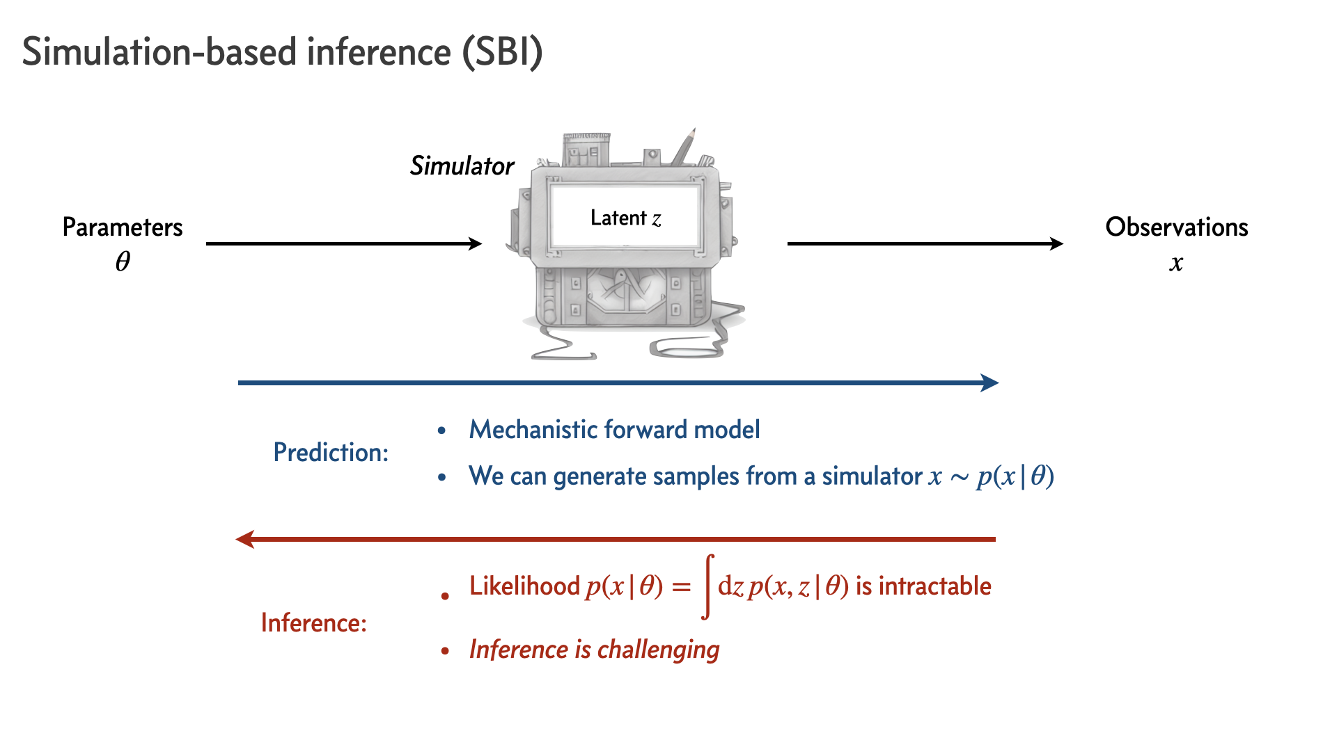
Probability of a simulation run depends jointly on observation and the stochastic latent variables $z$ of the simulator: $ p(x, z | \theta) $.

However, we only observe $x$, so the likelihood we need is marginalized over latent variables: $$ p(x|\theta) = \int p(x, z | \theta) dz = \int p(x | z, \theta) p(z | \theta) dz $$
$\Longrightarrow$ This marginal likelihood is intractable!

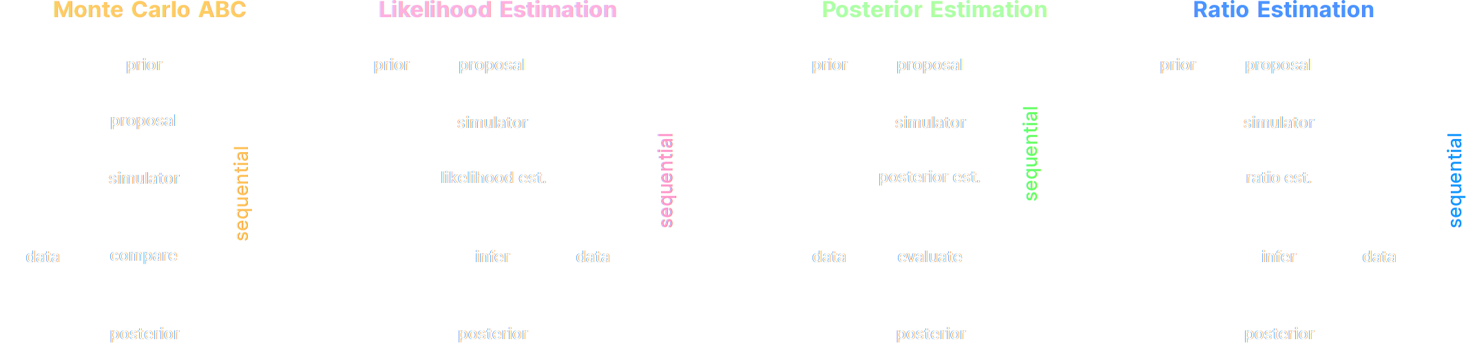
A variety of algorithms

Lueckmann, Boelts, Greenberg, Gonçalves, Macke (2021)

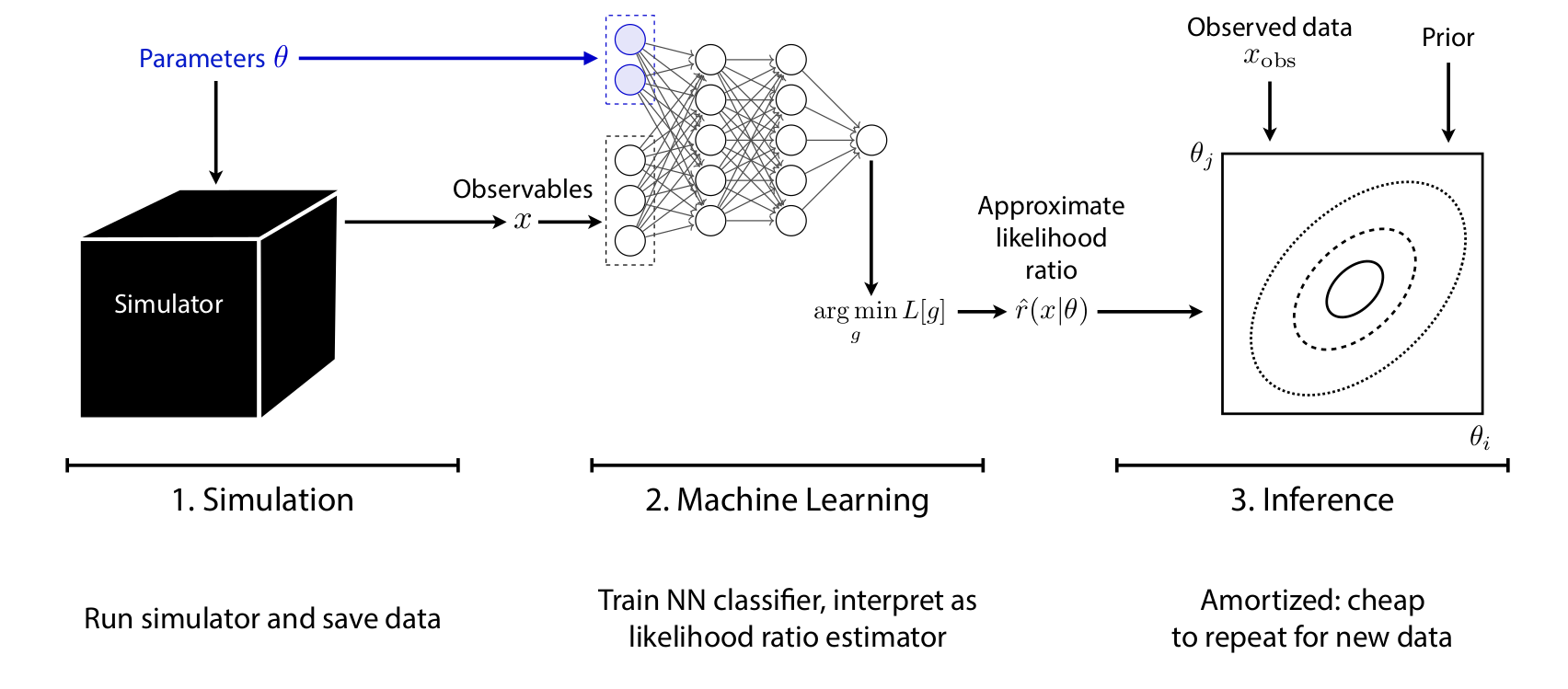
SBI with Marginal Neural Ratio Estimation

Information about $p(x|\theta)$ is implicitly accessed via a stochastic simulator, mapping: $\theta \rightarrow x$

Drawing parameters from the prior, $p(\theta)$, and calling the simulator → generate $N$ data-parameter pairs $\{(x_1, \theta_1), \dots, (x_N, \theta_N)\}$, drawn from the joint distribution $p(x, \theta)=p(x|\theta)p(\theta)$

Can also construct samples from the product of marginals $p(x)p(\theta)$, by randomly shuffling the data and parameters

Neural Ratio Estimation

Use these two sets of data-parameter pairs to train a neural network to estimate the ratio: $$ r(x ; \theta) \equiv \frac{p(x,\theta)}{p(x)p(\theta)} = \frac{p(x|\theta)}{p(x)} = \frac{p(\theta|x)}{p(\theta)} $$

$\Longrightarrow$ Determining $r(x ; \theta)$ is equivalent to determining the likelihood-to-evidence ratio or the posterior-to-prior ratio.

$\Longrightarrow$ Allows to obtain posterior samples by drawing samples from prior $p(\theta)$ and weighting them by $r(x ; \theta)$

Ratio computation

To compute $r(x ; \theta)$, train a binary classifier $d_{\phi}(x, \theta)$ ($\phi$ are the parameters of the neural network) to distinguish between samples from the joint and the product of marginals: $$ d_{\phi}(x, \theta) \approx \begin{cases} 1 & \text{if } (x, \theta) \sim p(x, \theta) \\ 0 & \text{if } (x, \theta) \sim p(x)p(\theta) \end{cases} $$
Learning problem → minimization of loss function (binary cross-entropy): $$ \ell \left[ d_{\phi}(x, \theta) \right] = - \int dx d\theta \, \left[ p(x, \theta) \ln d_{\phi}(x,\theta) + p(x)p(\theta) \ln (1-d_{\phi}(x,\theta)) \right] $$

Solution

$$ \boxed{d^*_{\phi}(x, \theta) = \sigma \left( \ln r(x ; \theta) \right) = \frac{p(x,\theta)}{p(x,\theta)+p(x)p(\theta)}} $$

$\Longrightarrow r(x ; \theta) = \frac{p(x,\theta)}{p(x)p(\theta)} \approx \frac{d_{\phi}(x, \theta)}{1-d_{\phi}(x, \theta)} = \hat{r}(x ; \theta)$

* Allows to directly estimate marginal posteriors by omitting parameters form network's input

LSS observables and synthetic data

Theoretical Predictions

Observables

Weak Lensing (WL): correlation between shear in the galaxy shapes
Galaxy Clustering (GC): correlation between galaxy positions
Cross-correlation between WL and GC (XC)

Obtain theoretical predictions on those by modeling their angular power spectra in multipole space, and dividing observations in redshift bins. Applying Limber approximation: $$ C_{ij}^{AB} = \int \frac{dz}{H(z) \, r^2(z)} W_i^A(z) W_j^B(z) P_{AB} \left( k_\ell(z), z \right) $$ where $W_i^A(z)$ are the window functions, $P_{AB}$ are the power spectra, and $k_\ell(z)$ is the wavenumber corresponding to the multipole $\ell$ at redshift $z$.

$C_\ell$ modelling

Galaxy clustering (doesn't trace total matter distr. directly)

$ W_i^g (z) = n_i^g(z) H(z), \,\, P_{gg} = b_g^2(z) P_{\delta \delta}(k,z) $

where $n_i^g(z)$: normalized distr. in $z$ of the observed galaxies in bin $i$, $b_g(z)$: galaxy bias (treat it as free nuisance param.)

Weak Lensing (traces directly the total matter distribution)

Intrinsic alignment: $C^{\epsilon \epsilon}_{ij}(\ell) = C^{\gamma \gamma}_{ij}(\ell) + C^{I \gamma}_{ij}(\ell) + C^{I I}_{ij}(\ell) $

$ W_i^\gamma (z) = \frac{3}{2} \Omega_m H_0^2 (1+z) r(z) \int_z^{z_{max}} dz' \frac{r(z')-r(z)}{r(z')} n_i^\gamma(z'), \,\, W_i^I(z) = n_i^\gamma(z) H(z) $

$P_{\gamma \gamma} = P_{\delta \delta} \left( k, z \right), \,\, P_{I I} = f^2_{\rm IA}(z) P_{\delta \delta} \left( k, z \right)$

Galaxy redshift distribution & Angular PS for photometric LSS probes ($3 \times 2$pt)

Noise and covariance

Creating synthetic data that mimic observations → need to model the observational uncertainty affecting the measurements, and how it propagates to the $C_\ell$s

Assume that the final measured spectra $C_\ell$ distributed following a multivariate Gaussian distribution, with a covariance matrix that they model as $$\begin{aligned} \mathbf{C}\left[C_{i j}^{A B}(\ell), C_{m n}^{A^{\prime} B^{\prime}}\left(\ell^{\prime}\right)\right]= & \frac{\delta_{\ell \ell^{\prime}}^K}{(2 \ell+1) f_{\text {sky }} \Delta \ell}\left\{\left[C_{i m}^{A A^{\prime}}(\ell)+N_{i m}^{A A^{\prime}}(\ell)\right]\left[C_{j n}^{B B^{\prime}}\left(\ell^{\prime}\right)+N_{j n}^{B B^{\prime}}\left(\ell^{\prime}\right)\right]+\right. \\ & {\left.\left[C_{i n}^{A B^{\prime}}(\ell)+N_{i n}^{A B^{\prime}}(\ell)\right]\left[C_{j m}^{B A^{\prime}}\left(\ell^{\prime}\right)+N_{j m}^{B A^{\prime}}\left(\ell^{\prime}\right)\right]\right\}, } \end{aligned}$$
Information on the observational uncertainties is encoded in the noise terms $N_{ij}^{AB}(\ell)$. Noise modelled as: $$N_{i j}^{A B}(\ell)= \begin{cases}\delta_{i j}^{\mathrm{K}} / \bar{n}_{\mathrm{g}}^i & A=B=\mathrm{g}, \\ \delta_{i j}^{\mathrm{K}} \sigma_\epsilon^2 / \bar{n}_{\mathrm{g}}^i & A=B=\epsilon \\ 0 & A \neq B \end{cases}$$

Results

Inference setup: Simulator

To perform the SBI analysis, require: a forward simulator and a neural network design.
The simulator has same statistical content as the multivariate Gaussian likelihood, and is defined as:

Simulator

Given the cosmological and nuisance parameters → compute each $C_{ij}^{AB}$, according to the equations above
Add a noise realization to each angular power spectrum, $\hat{C}_{ij}^{AB} = C_{ij}^{AB} + n_{ij}^{AB}$, where $n_{ij}^{AB}$ is drawn from the multivariate Gaussian $\mathcal{N}(0, \mathbf{C})$, with the covariance matrix $\mathbf{C}$ shown previously

Generate $5\times 10^4$ simulations by varying all cosmological and nuisance parameters $\{H_0, 100\omega_b, \omega_{\rm cdm}, n_s, \ln(10^{10}A_s)\} + \{ A_{\rm IA}, \eta_{\rm IA}, \sigma_{\rm IA}, b_1, \dots, b_{10} \}$.

Each parameter $\theta_i$ drawn from a uniform prior $\theta_i \sim \mathcal{U}\left( \left[ \theta_i^0 - 5 \sigma_i^F, \theta_i^0 + 5 \sigma_i^F \right] \right)$, where $\theta_i^0$ is the fiducial value and $\sigma_i^F$ is the fiducial error, estimated from the Fisher matrix as $\sigma_i^F = \left( F^{-1} \right)_{ii}^{1/2}$.

Network

$Relation between $\kappa$ and $\gamma$$

Data compression: pre-compress data using PCA
Inference

Output of trained network: different estimated ratios for the parameters of interest.

Forecast posteriors for $\Lambda$CDM

MNRE and MCMC posteriors are in excellent agreement

MNRE results in a speedup factor of $\sim$ 40

MNRE directly estimates the marginal posteriors $p(\theta_i|x)$ and $p(\theta_i, \theta_j|x)$ $\Longrightarrow$ requires far fewer simulation runs that sampling the full joint posterior and marginalizing

Generation of simulations with MNRE can be fully parallelized, while MCMC is inherently sequential

MNRE can be also used to evaluate consistency and get information about e.g. systematics and astrophysics

Forecast posteriors for decaying dark matter

MNRE can be applied to accelerate the inference of $\Lambda$CDM extensions, having significantly non-Gaussian posteriors.

$\Lambda$DDM: model where DM is allowed to decay into a massless and a massive particle.

Characterized by two extra parameters: the DM decay rate $\Gamma$ and the velocity kick $v_{\rm k}$ received by the warm decay product.

Here, they vary not only the $\Lambda$CDM and nuisance parameters, but also the two new parameters.

MNRE and MCMC posteriors are in very good agreement

MNRE can be easily applied to test alternative models exhibiting significantly non-Gaussian posteriors & Stage IV surveys can improve the bounds on $\Lambda$DDM by up to 1 order of magnitude.

Conclusions and outlook

MNRE can be used to optimize cosmological parameter inference from upcoming Stage IV surveys.

Benefits compared to LBI

Does not need to assume a possibly incorrect functional form for the likelihood, only to generate samples from it.

Directly estimates the marginal posteriors of interest, without the need to sample the full joint posterior $\Longrightarrow$ much more efficient and flexible than conventional MCMC.

The generation of simulations can be fully parallelized, while MCMC is inherently sequential.

Allows to perform statistical consistency checks, e.g. coverage tests, which are usually unfeasible with MCMC.

Conclusions and outlook

To illustrate this, they focused on the photometric $3\times 2$pt statistics measured at 10 tomographic bins that they modelled with a 17-dim cosmological+nuisance parameter space.

Findings

Able to accurately reconstruct the posterior of all $\Lambda$CDM and nuisance parameters, with 1-2 orders of magnitude speedup compared to MCMC.

Showed that MNRE performs equally well when posteriors are significantly non-Gaussian, as in the case of $\Lambda$DDM. Again, they find posteriors in excellent agreement with MCMC at a fraction of the computational cost.

Future work:

Extend the pipeline to include other LSS observables
Here they have used 2pt statistics, that capture only a fraction of the information content in the dat → explore field level inference, to extract all information available in higher order statistics.